autoPROC Documentation : Computing and visualising predictions

Contents

• Introduction
• Computation of positions and shapes of reflections with simcal_predict
• Visualisation with GPX2

Introduction

Computation of positions and shapes of reflections with simcal_predict

At the first step, a pseudo-3D covariance matrix between spot position coordinates and diffraction angle is computed analytically (which has been confirmed to agree with the shape information that can be obtained by ray-tracing simulation). This is done by computing a 3x12 Jacobian matrix, the first two rows of which are the Jacobians of the spot coordinates, the third row is a gradient of the diffraction angle. Derivatives are taken w.r.t. the following twelve variables: cell orientation (3), cell axis lengths (3), cell angles (3), beam orientation (2) and wavelength (1).

Next, the error model for those variables is assembled by using user-supplied e.s.d.'s for those variables and, optionally, correlations between the three angles used to simulate crystal mis-orientations (mosaicity model as proposed by Kay Diederichs, 2009). These e.s.d.'s are the same as used to control random-number generation (RNG) during ray-tracing. The model is either purely diagonal or, if correlations mentioned above are given, a block diagonal one. Together with the computed Jacobian, this error model is used in the propagation-of-error formula to compute a final 3x3 covariance matrix of the variables of interest.

This matrix is always dense, even if the error model used is diagonal. The method to plot the image-by-image confidence ellipses with GPX2 is to decompose the initial Gaussian into a product of conditional and marginal distributions, where conditioning is done on the third variable (the mid-frame values of the frames on which the spot is visible). This decomposition is particularly simple, as one sub-block of the original covariance matrix is of size just 1x1. Choosing the right Schur complement to perform the required matrix inversion makes the task very easy. Finally, only the conditional part, this time a true 2D-ellipse, can be plotted. The coordinates of its centre depend explicitly on conditioning information, so the movement of ellipses from frame to frame is naturally achieved.

The covariance matrix of this ellipse is still fixed. The change in size is achieved by combining a specified confidence-level parameter (the initial size) with the marginal part of the Gaussian to introduce a correction factor explicitly depending on the conditioning. If this parameter becomes negative, it means that the conditioning is invoking values outside the initial ellipsoid, and the ellipse is not displayed.

Geometrically, this procedure is equivalent to computing the intersection between the original ellipsoid and a plane perpendicular to the axis used in conditioning. Note that in our case this variable is not precisely Cartesian, it represents a linearised angular variable. The intersection of the 3D-ellipsoid with a plane is a 2D-ellipse, if it exist.

The computation of the 3D covariance matrix is done in simcal_predict. The conditioning algorithm that then produces the 2D-ellipses has been ported into GPX2 in order to perform this task dynamically.

The invocation of simcal_predict is done within autoPROC as part of data processing and therefore not directly exposed to the user.

Visualisation with GPX2

GPX2 can be started with a diffraction image given on the command line, e.g.

gpx2 some.cbf

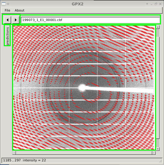
The window will show the diffraction image itself, buttons to move from one image to the next, a text box to type the image name directly and an (initially hidden) area called "predictions". The window itself can be enlarged to any size required.

Navigating within the diffraction image panel is done using the mouse (ideally one with a mouse-wheel):

• the mouse-wheel will zoom in and out at the current center defined by the mouse pointer
• panning is done with the left mouse button

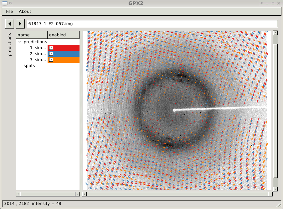
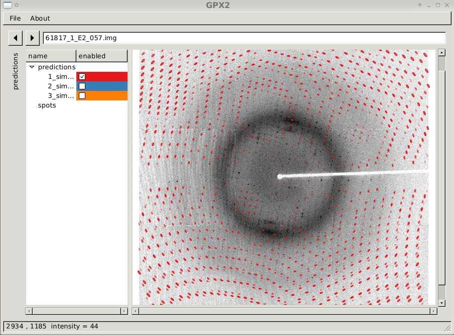
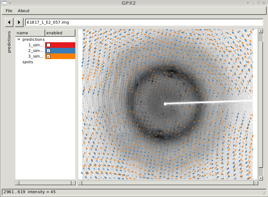
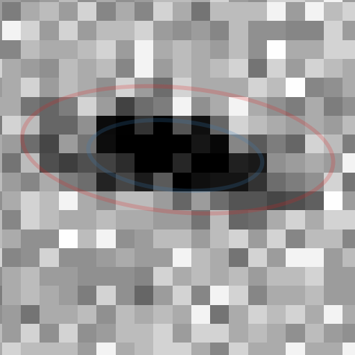
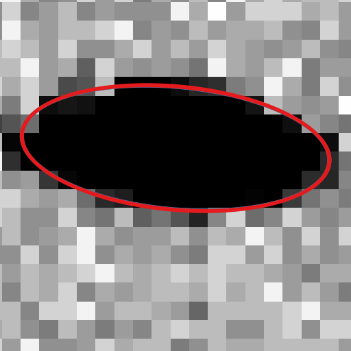
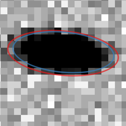
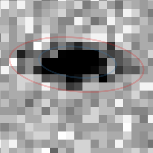
Predicted spot positions and shapes are presented through ellipses:

• the size of each ellipse is a 2D representation of the 3D spot shape computed by simcal_predict as it is intersected by the diffraction image during rotation.
• the opacity is proportional to the partiality of the reflection on the given image

Usually a user will not start GPX2 directly, but through one of the "gpx.sh" scripts generated as part of an autoPROC run. These scripts take care of generating the appropriate input to simcal_predict (via the xparm2simin tool) at different stages of data processing: initial indexing, multi-lattice cases, first integration and final integration. They provide command-line arguments for selecting specific indexing solutions or create plots with or without predictions.