Content:
Introduction
The first thing to always check is the image header - to see that imginfo gives the expected results. Here we have
% imginfo XXXX_3_00001.cbf
################# File = XXXX_3_00001.cbf

>>> Image format detected as Pilatus

===== Header information:
date                                = XX XXX XXXX XX:XX:XX
exposure time             [seconds] = 4.998
distance                       [mm] = 500000.000
wavelength                      [A] = 1.000000
Phi-angle                  [degree] = 0.000
Omega-angle (start, end)   [degree] = 0.000 0.500
Oscillation-angle in Omega [degree] = 0.500
Kappa-angle                [degree] = 0.000
2-Theta angle              [degree] = 0.000
Pixel size in X                [mm] = 0.172000
Pixel size in Y                [mm] = 0.172000
Number of pixels in X               = 2463
Number of pixels in Y               = 2527
Beam centre in X               [mm] = 221.020
Beam centre in X            [pixel] = 1285.000
Beam centre in Y               [mm] = 224.460
Beam centre in Y            [pixel] = 1305.000
Overload value                      = 1095344
which looks mostly correct - apart from the distance. This (now fixed?) problem is due to the distance being written in mm into the image header (when the standard way is to give it in metres).
So we need a little wrapper script to fix that:
Running now
% /where/ever/imginfo_X25old.sh XXXX_3_00001.cbf
gives the correct distance (500 mm).
Simple, initial run
We can either run
% process imginfo=/where/ever/imginfo_X25old.sh -d 01 | tee 01.lis
in the directories with the images, or specify the image directory explicitely (and run it anywhere):
% process imginfo=/where/ever/imginfo_X25old.sh -I /some/where/images -d 01 | tee 01.lis
This finds the 400 images and starts processing (with all output going into a subdirectory):
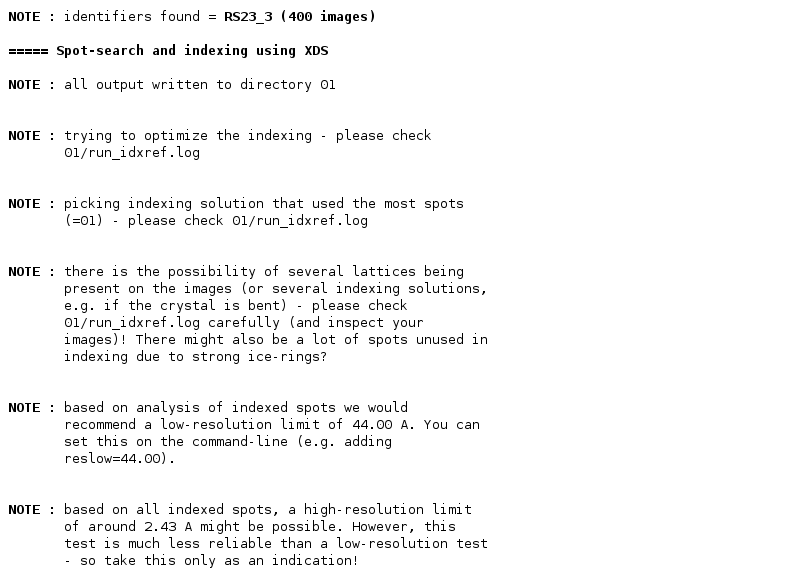
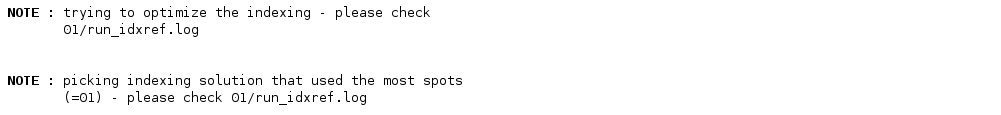
There seems to be an issue with the indexing: it wasn't able to index most found spots with a good solution. So it goes into some 'iterative indexing' and reports possible reasons for that problem (multiple lattices, ice-rings etc). So we should have a closer look at this later!
It also mentions resolution limits (both low- and high-resolution) based on the indexed spots. This can be used as a rough indication, since integration might extract useful intensities even for very weak reflections that aren't classified as spots at this point.
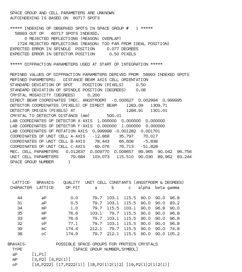
Next details of the found indexing solution are given:
This looks like a good solution:
- refined distance (500.01 mm) stays close to input distance (500.00 mm)
- low standard deviations on spot position (0.5 pixels) and spindle position (0.08 degree).
A list of possible lattices is given: here the mP lattice (monoclinic primitive) seems the most likely candidate. However, autoPROC will run integration first in P1 and decide on the most likely lattice and spacegroup only after the full dataset has been integrated. One could enforce a specific spacegroup e.g. with
% process symm=P2 ...
or
% process symm=P21 cell="80 116 103 90 97 90" ...
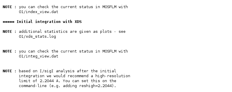
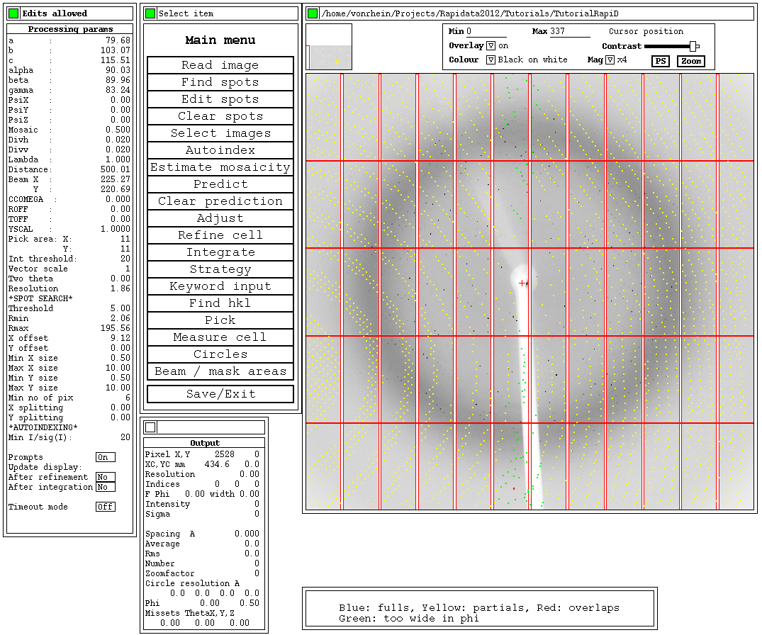
At various points, autoPROC will report the possibility to visualise the current status via MOSFLM:
One can load those predictions into MOSFLM using e.g.
% ipmosflm < 01/index_view.dat
Within that (old) MOSFLM display, you can see the predictions via the Predict button:
The high-resolution estimation has been updated after this integration - and is a little bit higher than initially (which was based on spots alone).
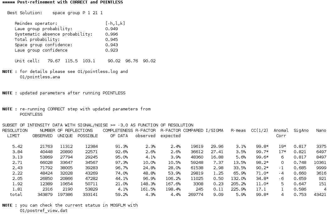
The next step is the decision on the most likely spacegroup: this is done using POINTLESS:
All scores for the various decisions are very high (above 0.9): so this is a fairly confident vote for P21. However, it is advisable to still check the POINTLESS log-file in detail for
- what's the resolution of accepted reflections for the spacegroup determination? If this is too low, it can easily miss or missassign some symmetry element.
- are there enough axial reflections to decide on screw components?
- any indication of twinning?
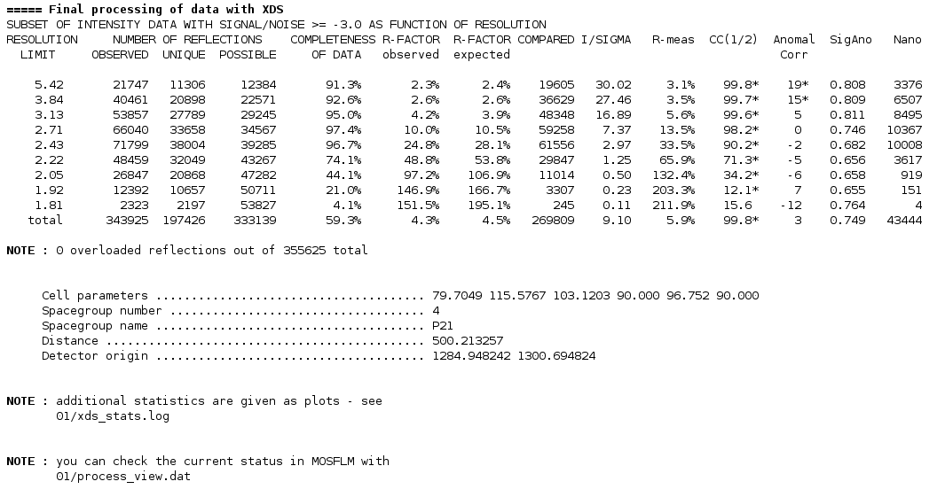
Once a decision about symmetry has been made, the last step of XDS (CORRECT) is re-run and the first table with merging statistics is shown.
Using the updated (post-refined) parameters and the newly assigned spacegroup, a second round of integration is done:
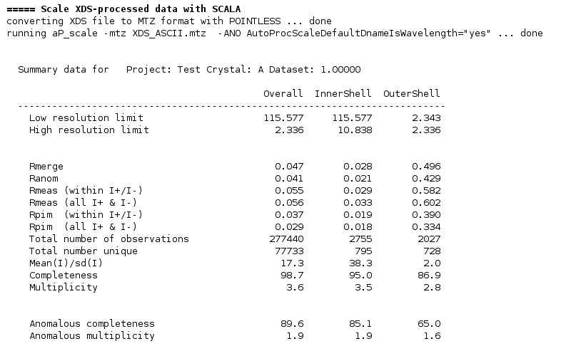
Finally, the data is scaled and merged using SCALA:
The scaling module aP_scale automatically decides on an apropriate high-resolution cut-off (based on R-factors, completeness and I/sigI values).
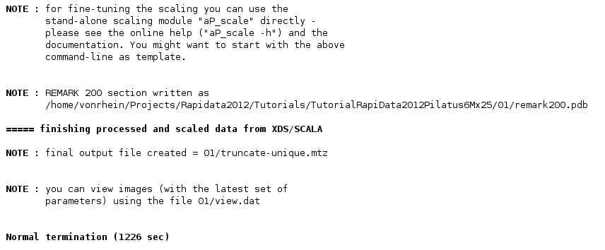
To finalise processing with autoPROC, a full REMARK 200 section is written and the intensities are converted into amplitudes:
Additional observations
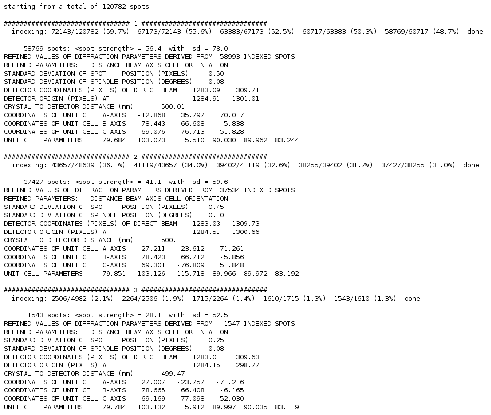
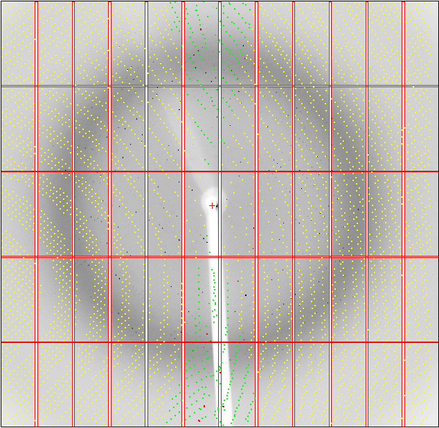
What are the interesting bits of information here? Let's first have a look at the message about indexing problems:
Looking into details of 01/run_idxref.log:
- the first indexing solution uses nearly 50% of found spots
- but the second solution still uses nearly a third of spots
- the next solutions can be ignored, since they use only very few spots and are probably noise.
So what is the reason for those two distinct indexing solutions? Let's compare the two orientations with
% cmpmat 01/01_XPARM.XDS 01/02_XPARM.XDS
gives
So a nearly 180-degree rotation between the two orientations. Can we visualise this? Yes - with
% cd 01
% ipmosflm < 01_tomos.dat &
% ipmosflm < 02_tomos.dat &
This shows clearly the two lattices, with each indexing solution only predicting part of the spots visible.