TutorialRapiData2023

Content:

• Introduction

• 7RIS
• Processing Calcium dataset with autoPROC
• Processing Holmium dataset with autoPROC
• Experimental phasing with SHARP/autoSHARP

---

Introduction

These notes here are specifc for the RapiData 2023 workshop at SSRL. We assume that you know how to (1) connect to NX/NoMachine, (2) start a terminal on one of the processing machines and (3) have some basic familiarity with the command-line.

If you opened a terminal on one of the processing machines, all our software should be setup correctly. Otherwise you might need to run

    module load ccp4
    module load xds
    module load autoproc

in order to have a correct setup for our software. In either case, you should now be able to see the online help via

    process -h

A PDF with the most important (or commonly used) command-line arguments is available here.

If you don't have your own data available for running autoPROC, you can have a look at some example data (mostly data deposited with PDB entries by various users): these are in

/data/rapidata2/SampleData2023

with a separate directory for each project (PDB identifier). In most you will find a subdirectory Images (if the raw diffraction data is available).

---

7RIS

There are two datasets available for this PDB entry:

• one containing Calcium (used for refinement): /data/rapidata2/SampleData2023/7ris/Images/Ca
• another one containing Holmium (used for SAD phasing): /data/rapidata2/SampleData2023/7ris/Images/Ho

For the tutorial it would be best if you created a fresh directory - e.g. via

    mkdir -p ~/rapidata2023/7RIS

and then go there:

    cd ~/rapidata2023/7RIS

Make sure you are on one of the fast processing nodes, i.e.

    hostname

returns something containing pxprocNN (with NN being the node number you are on).

Processing Calcium dataset with autoPROC

We can just run

    process -I /data/rapidata2/SampleData2023/7ris/Images/Ca -d Ca.01 | tee Ca.01.lis

Here

• -I <directory> tells autoPROC where the images are
• -d <directory> tells it into what (sub)directory all output should go
• the | tee Ca.01.lis construct pipes (vertical bar) standard output into the tee command - with the name of the file all standard output should be saved to using the same name as the directory -d with the extension .lis (you could use a different extension if you want (.log, .out or .txt) if you want: it doesn't matter as long as you have some consistency in your naming convention)

You will now see a lot of text in your terminal, which can be very useful to read since it contains a lot of information. However, it passes quite quickly and scrolling up and down can be tedious. No problem, since we also saved the output into a file (via that tee command above) - so nothing is lost.

The better way of looking at autoPROC results is the so-called "summary.html" file it generates automatically, and which can be found inside the directory specified by the -d flag. So if you followed the suggestions above, you should find it at ~/rapidata2023/7RIS/Ca.01/summary.html and you can open it e.g. via the command

    firefox ~/rapidata2023/7RIS/Ca.01/summary.html

Remember to hit the "Reload" button (or Ctrl-R) from time to time: that file is being written to by the currently running process and we might want to refresh what we see. As soon as you see a proper menu on the left hand side (in that slightly grey panel) the job will be finished ... hopefully without any error.

The information in the HTML document should be fairly clear: you will see notes, sometimes warnings and various graphs with explanations (and there are links to only documentation available as well). Some sections are "hidden" by default: symbolised by the little green box with a "+" sign: clicking on it will expand that section and provide you with more information and plots.

The overall sequence of autoPROC steps are

• preparation (reading image headers, database lookup etc)
• spot search (on all images up to 360 degree of data)
• iterative indexing (including analysis of multiple indexing solution, ice-rings etc)
• analysis for image ranges without spots (if e.g. crystal moved in and out of the beam)
• initial integration (in P1 - unless otherwise defined by user)
• determination of most likely space group
• additional analysis for poor image ranges (radiation damage, poor diffraction quality etc)
• second (or sometimes more) integration now with the determined SG set (cell restraints)
• scaling
• analysis for anisotropy via STARANISO
• final reporting (PDF reports) and generation of merged reflection data (MTZ and SCA files), unmerged reflection data, deposition-ready mmCIF files and data quality metrics in different format (XML, ASCII files).

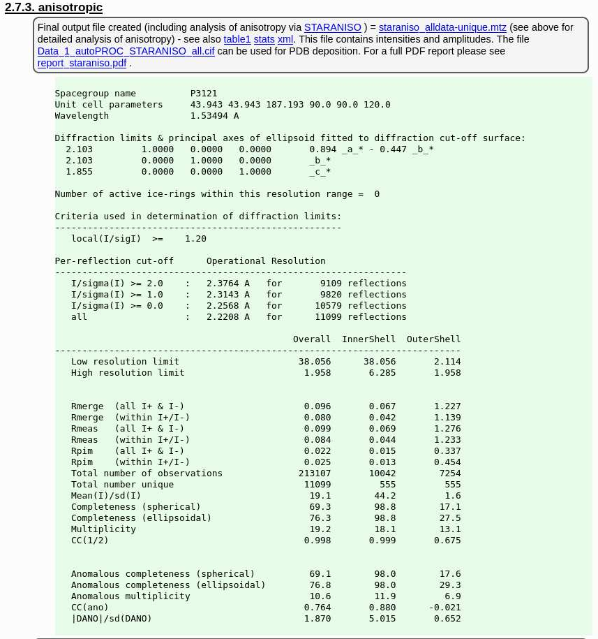
At the end of this autoPROC job you should have quite nice data - e.g. visible via the STARANISO analysis

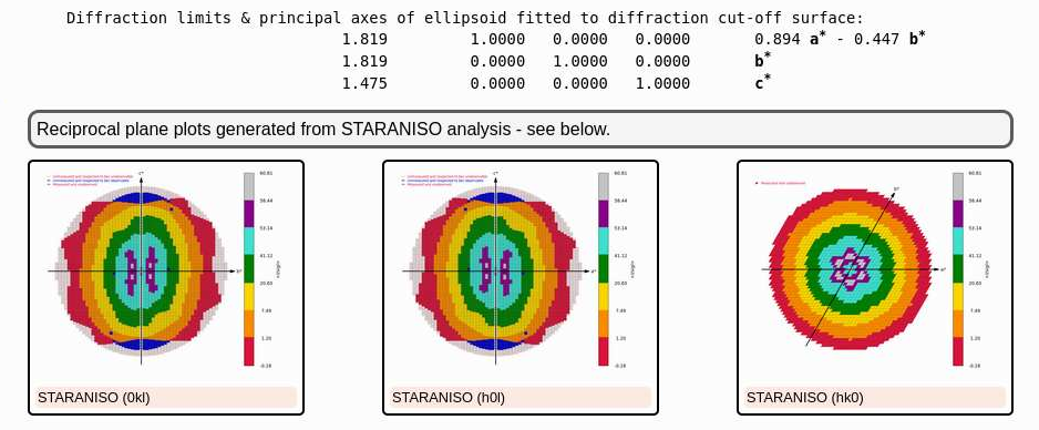and the final set of data-quality metrics

Processing Holmium dataset with autoPROC

We could now process the Holmium dataset in the same way - and we should do so if we didn't know anything else about it. But let's assume that this is just a replacement of the calcium ion and that the crystal form stays basically the same. Then we could use the just processed data as a reference in order to

• ensure the same space group and cell
• use (through transfer and completion) the same set of test-set flags (in case we want to transfer models between datasets and want to have an unbiased Rfree value for comparison)
• ensure that datasets are consistently index (see e.g. here)

So let's run

    process \
      -I /data/rapidata2/SampleData2023/7ris/Images/Ho \
      -ref Ca.01/staraniso_alldata-unique.mtz \
      -d Ho.01 | tee Ho.01.lis

For better readability we used a backslash (and then a newline) - standard shell syntax to signal continuation (you can still cut-n-paste the above into a terminal as-is).

Now we get an idea about the quality of that dataset:

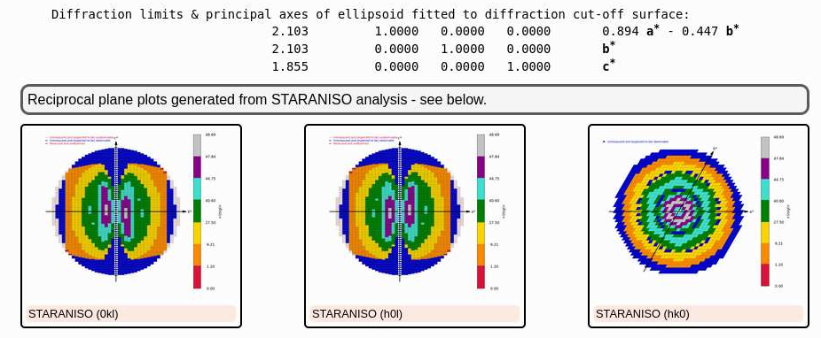(because of the longer wavelength and the long c-axis, the detector could not be moved closer to record the higher diffraction data - as was possible for the Calcium dataset) and the final set of data-quality metrics

Experimental phasing with SHARP/autoSHARP

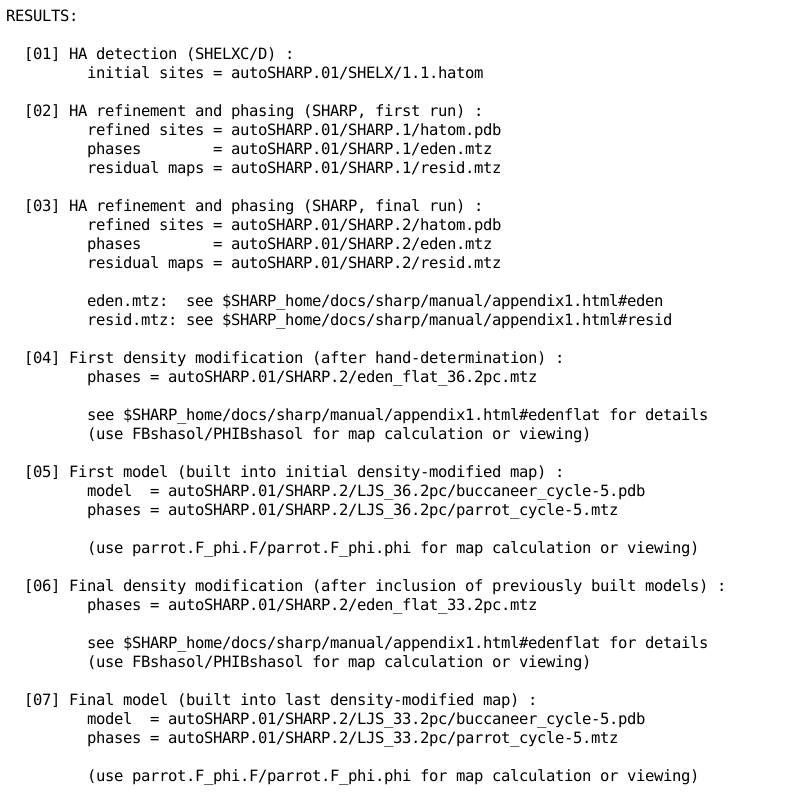
Because we have (strong) anomalous signal in the Holmium dataset, we can run SAD phasing. First we need to get the sequence file via

    wget -O 7ris.seq https://www.rcsb.org/fasta/entry/7RIS

than we can run

    run_autoSHARP.sh \
      -seq 7ris.seq \
      -ha "Ho" -nsit 1 \
      -wvl 1.53494 peak \
      -mtz Ho.01/staraniso_alldata-unique.mtz \
      -nowarp \
      -d autoSHARP.01 | tee autoSHARP.01.lis

The above is using nearly all defaults for SAD phasing (see also run_autoSHARP.sh -h or the PDF cheat-sheet) - apart from the -nowarp flag: this is only to skip the final ARP/wARP model building step to get faster to an already sensible result.

While the job is running you could load the HTML it references (on standard output) - or wait till it is finished. You should then see something like:

and several instructions/suggestions like

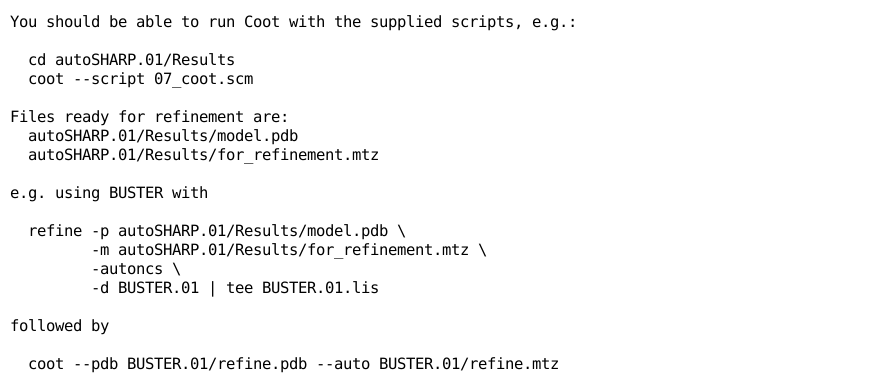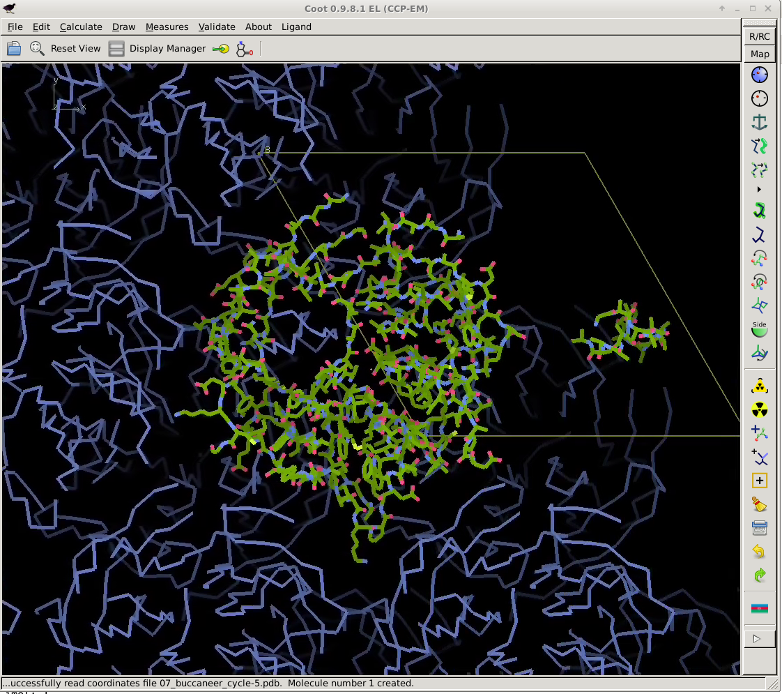
Following one of those, namely

   cd autoSHARP.01/Results
   coot --script 07_coot.scm

allows you to check the current status of the structure solution and initial model building:

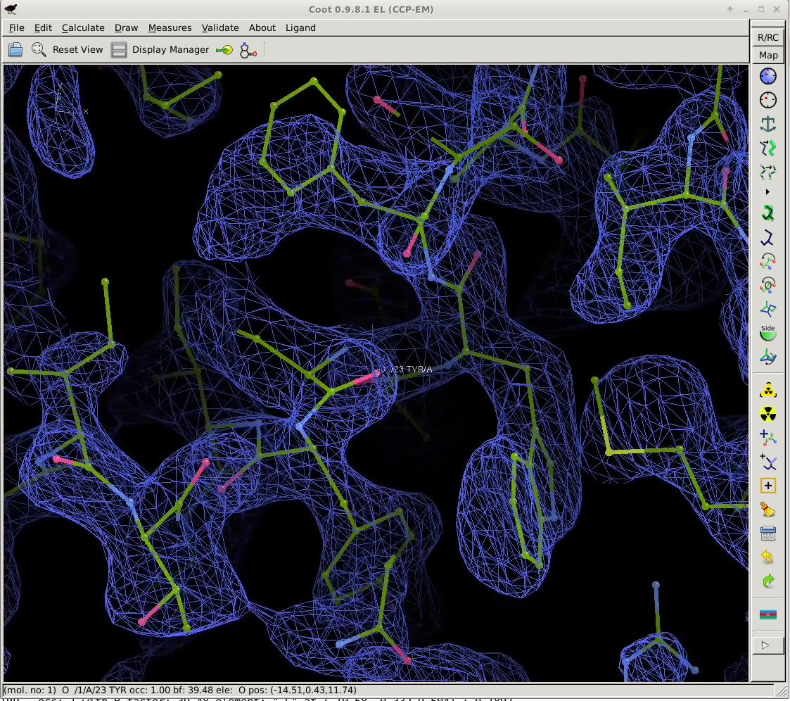That model might not yet be in a state for going directly into refinement (it is after all a quick initial build only), but it shows that the structure can be solved by SAD phasing (as it was done originally) and that the initial model should provide a good starting point for completion - either manually or via some other tools/programs.