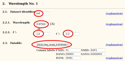
The Se-MET data was collected as interleaved wavelengths (inflection and high-energy remote). A Fluorescence scan gave f'/f" values of
| Dataset | Wavelength | f' | f" |
| hrem | 0.91162 | -1.8 | 3.3 |
| infl | 0.97934 | -11 | 3.0 |
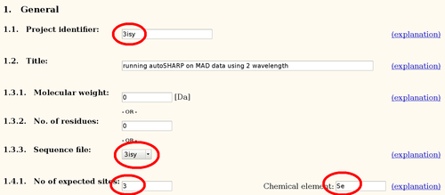
The sequence (120 residues) contains 3 methionines - 3isy.pir:
GMENQEVVLS IDAIQEPEQI KFNMSLKNQS ERAIEFQFST GQKFELVVYD
SEHKERYRYS KEKMFTQAFQ NLTLESGETY DFSDVWKEVP EPGTYEVKVT
FKGRAENLKQ VQAVQQFEVK
Data was processed with autoPROC, resulting in two files:
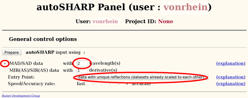
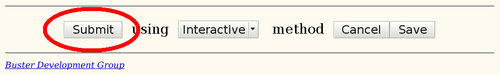
It is always best to start a new project by running the fully automated autoSHARP pipeline (Vonrhein, C., Blanc, E., Roversi, P. & Bricogne, G. (2007). Automated structure solution with autoSHARP. Methods Mol Biol 364, 215-30). From the results it is easily possible to run follow-up calculations to fine tune the heavy-atom model in SHARP, change density modification parameters, add additional datasets or include an existing partial model.
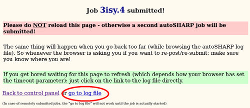
The main autoSHARP logfile is a simple HTML document:
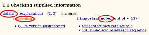
Some warnings might be unavoidable, a typical example is the warning about a (potentially) unsupported CCP4 version. Since a specific SHARP/autoSHARP release was tested against the CCP4 version available at the time, autoSHARP will inform the user if a newer version is actually used during the run. However, it is very unlikely that this would have a significant effect upon the results if it is only an updated patch release of CCP4 (e.g. 6.1.13 when 6.1.1 was current at the time of the SHARP/autoSHARP release).
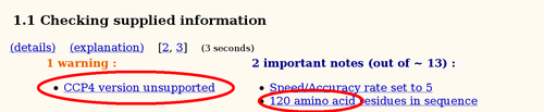
Several notes towards the beginning of an autoSHARP job seem rather dull and trivial (like the number of residues). Nevertheless, those are good indicators that simple things like file format conversions have been done correctly (e.g. creating the PIR-formatted sequence file).
Each of those notes/warnings are hyperlinks to the details page where some additional information and/or explanation (usually as a link to the online manual) can be found.
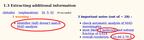
The warning about the MAD analysis is rather unusual: clicking on that hyperlink will give some more details. This analysis is based on mainly on user-supplied f' and f" values. Those values (see target history from JCSG) should be very accurate if determined through a fluorescence scan. Maybe some misassignment of datasets/wavelengths occured?
An analysis of asymmetric unit content (using Matthews coefficient) will show the most likely number of molecules given the monomer sequence. It is important that the sequence and the number of expected heavy atom sites are in sync: autoSHARP will multiply both the sequence and the number of sites to search for based on this analysis. Therefore, in most cases the monomer sequence and the number of expected sites per monomer should be given.
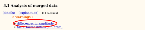
Some possible warnings relate to the comparison of different datasets (here the two wavelengths of the MAD experiment): a significant amount of differences in amplitudes - especially if those are mostly low-resolution reflections - might point to problems in low-resolution data processing (beam stop masking) or scaling with very low multiplicity.
Even only a few outlier reflections can have a big impact on the success of the structure solution, mainly at the heavy atom detection step (were normalised structure factors, oe E values, are used). Since large outliers usually occur at low resolution (where the reflexions are strongest), great care during data processing should be taken especially at the low resolution end.
Experimental phasing using a heavy atom model is obviously only possible if one can find this heavy atom substructure. As a general rule, one often needs much better heavy atom signal to find the sites in the first place, than is needed for phasing and solving the structure once a correct set of positions is available. For that reason, two distinct steps are required at this point:
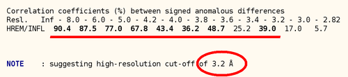
In the case of a MAD dataset, the most reliable statistic for determining the high-resolution cut up to which a good heavy atom signal is available, is the correlation between anomalous differences. Here we can see that there seems to be good anomalous signal to about 3.2A (statistics from SHELXC):
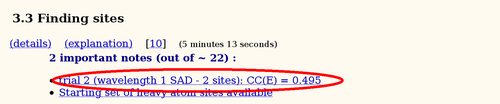
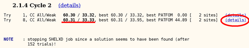
autoSHARP uses this statistic to automatically cut the resolution used in heavy atom detection. The currently best trial solution from SHELXD is shown:
For this Se-MET experiment one would assume that all Se sites are fully occupied (with some caveat: N-terminal Met could be disordered, other Met could have alternate conformations or the Se-MET incorporation wasn't complete). Therefore, the plot of found sites should show the number of expected sites with high occupancy, followed by a clear drop when wrong sites (noise) start to appear:
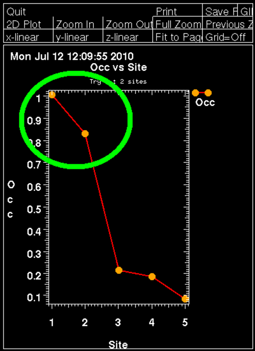
Here we can clearly see two mayor sites - the N-terminal MET is probably disordered (the deposited PDB file has the first 3 residues missing).
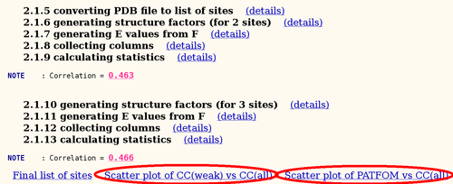
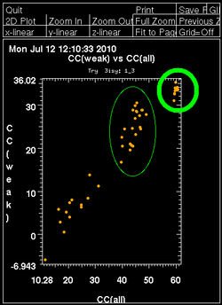
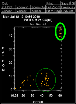
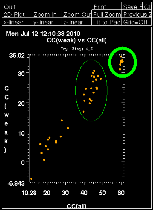
Once autoSHARP thinks that a reasonable solution has been found, additional statistics are provided as well as scatter plots for pairs of scores: CC(weak) vs CC(all) and PATFOM vs CC(all). The idea is that the substructure detection will lead a number of correct solutions as well as some wrong solutions - and that those two classes will be well separated in those quality scores. If these plots show no clear separation of clusters (or at least one solution significantly better than the majority), it is unlikely that the found substructure is actually correct - unless one has an extremely strong heavy atom signal and basically all solutions are correct.
It is important to have some confidence in the substructure solution, since otherwise the following steps can lead to a very large number of phase sets that will be difficult to judge and analyse.
Once a set of heavy atom positions are found, their parameters (position, occupancy and B-factor) as well as scale and non-isomorphism parameters will be refined in SHARP. Ideally, all initial sites should have their parameters refined to meaningful values resulting in a set of good phases:
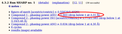
A very useful criteria to judge the quality of a set of phases is the resolution at which the phasing power drops below one. This should be a value similar to other criteria of heavy atom signal quality (correlation of anomalous differences or Rmeas/Rmeas0 comparison and correlation between half-sets as given in SCALA).
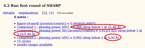
In the example here there is clearly something wrong with the anomalous phasing power for the first wavelength (infl): it gets very poor values and basically no phase information. What could be the reason for that becomes clearer in the next step.
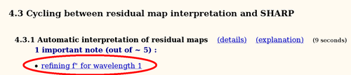
To adjust the current heavy atom model, the so-called "residual maps" (log-likelihood gradient maps) are analysed to e.g. detect wrong or additional sites. Here we get a clear indication of a mistake in the f" value for the inflection dataset:
The more detailed exlpanation
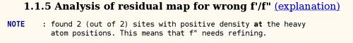
shows that the f" value is probably too low (since the residual map has positive peaks at the heavy atom positions). After switching on the refinement of f" for the first (infl) wavelength, the resulting statistics look much better:
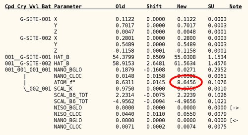
The detailed list of parameters shows that the initial value of 3.0 was definitely too low and that a value around 8.6 is much more likely. Furthermore, the local non-isomorphism parameter on anomalous differences (NANO_CLOC) refines from a rather large value of 0.4 to basically zero.
Maybe the wavelength was closer to the peak than to the inflection point? Fortunately, the JCSG database contains the fluorescence scan:
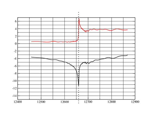
One can see how close the inflection and peak actually are:
   Energy          f'             f"
-------------------------------------------------------------
  12659.20      -11.12677       3.097779
  12659.51      -11.24010       3.756472  <<< infl 0.97938 A
  12659.82      -11.17152       4.478636
  12660.13      -10.90237       5.190691
  12660.44      -10.44393       5.819074
  12660.75      -9.839978       6.300265
  12661.07      -9.155026       6.587479
  12661.38      -8.467686       6.670717 <<< peak 0.979239 A
  12661.69      -7.850429       6.573413
The wavelength value of 0.97934 (recorded in the image header or in the JCSG target history) might indicate an energy slightly off the inflection point and more towards the peak.
Once a set of experimental phases is available, the decision about the correct handedness of the heavy atom substructure (and corresponding enantiomeric space group) needs to be made. In nearly all cases, the heavy atom solution would also be consistent with the data after inverting all heavy atom positions through the origin. For several spacegroup this would also result in a change to the enantiomorph (P41 to P43 etc). Important: there are only ever two possibilities to test since a change of substructure handedness automatically means a change to the enantiomeric space group.
The two phase sets should be easily distinguishable when calculating electron density maps: one should give a chemically sensible map whereas the other should be basically just noise. To distinguish those two cases, we use a single cycle of density modification to compare some statistics (which are combined into a 'score'):
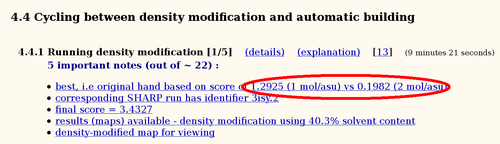
There is no doubt that in this case the original hand is significantly better than the inverted hand. Often the difference in scores isn't that obvious, but some difference should still be visible: if the two scores are more or less identical it is unlikely that the current heavy atom model is actually correct.
After deciding on the hand (and therefore phase set), these experimental phases are improved through standard density modification procedures using solvent flipping. A series of such runs is performed with varying values of solvent content to get the best map possible.
The hopefully best electron density map after density modification is used for automatic model building using ARP/wARP:
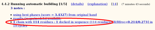
Of the 120 residues, 114 can be built into this 2.8A map (the deposited PDB file contains 117 residues).
At the end of an autoSHARP run, some references for used software or methods are given. These could be used directly in any manuscript using results from SHARP/autoSHARP.
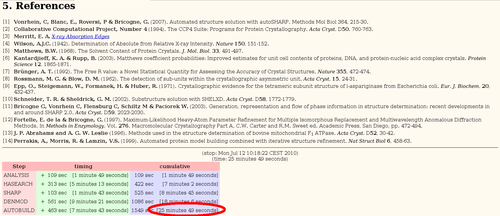
There is also a little table summarizing the time spent in each step. As one can see, the initial analysis and the parameter refinement in SHARP are often the fastest steps. More time is spent in the heavy atom detection and especially density modification and model building towards the end. The timings here are for a Dell latitude D630 with Core2 Duo T7700 (2.40GHz).
To view the results, the various links can be used, e.g.
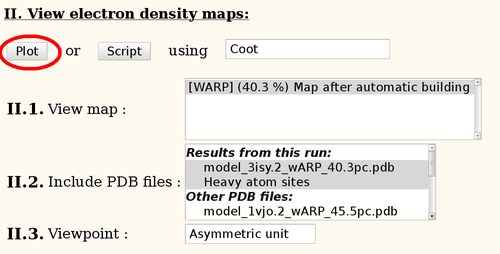
This should start Coot with the automatically built model and the corresponding map. Note: this is run in a temporary directory which is deleted after exiting Coot - so be sure to save any manual modifications.