Direct use of weighted Quantum Chemical Energy for ligands in BUSTER refinement
QM introductory tutorial example:
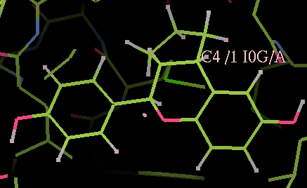
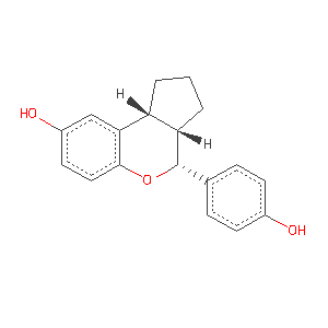
benzopyran ligand bound to 2i0g
Contents
Background
- For an introduction to the ideas behind the weighted-QM energy as a restraint function for ligands see AutobusterLigandQMIntroduction.
- Here we will use the method to treat the benzopyran ligand I0G in the estrogen receptor beta structure 2i0g.
- 2i0g is a structure of the estrogen receptor beta with the I0G ligand bound.
- The structure was solved by Yong Wang (Eli Lilly) and diffracts to 2.5Å resolution. It has respectable geometry as gauged by MolProbity and its reciprocal space correlation coefficient plot looks very reasonable.
- The receptor has 2-fold NCS with a ligand bound in both sites. The density for the ligands is clear for the resolution.
- This tutorial shows that weighted-QM energy ligand restraints yield a conformation similar to that obtained from a GRADE dictionary. In addition the QM method indicates that the ligand is slightly strained on binding, with the phenolic ring being rotated from the unbound state.
Starting Files
- The PDB and MTZ files were obtained by using collect.pl, see AutoBusterExampleUsingPDB.
- The GRADE dictionary for the ligand I0G, based on Mogul CSD information, was generated by:
grade_PDB_ligand I0G
(A) Preparation: add hydrogen atoms to the ligand(s)
- To run the QM method it is essential that your ligand is chemically complete, in particular its hydrogen atoms must be present. In 2i0g.pdb the two copies of I0G do not have hydrogen atoms modelled so we must first add them.
- To do this run the hydrogenate tool:
hydrogenate -p 2i0g.pdb \
           -l I0G.grade_PDB_ligand.cif \
           -ligonly -zero \
           -o 2i0g_addhI0G.pdb
- hydrogenate
- Uses Richardsons' Lab reduce program so this must be on your PATH. See http://kinemage.biochem.duke.edu/software/reduce.php for information (it is also included in MolProbity).
- hydrogenate understands the hydrogen atoms specified in a Refmac/CCP4-style CIF restraint dictionary.
- The -ligonly option means add hydrogen atoms only to the ligand and not the protein.
- The -zero option means assign zero occupancy to the hydrogen atoms added. This is recommended because at this resolution explicit full occupancy hydrogen atoms are not recommended.
- The -o option specifies the output filename. Use COOT to check that the hydrogen atoms have been added correctly:
coot -p 2i0g_addhI0G.pdb
- You should see that both the A and B copies of the I0G ligand have hydrogen atoms added:
(B) Refine with -qm I0G -l I0G.grade_PDB_ligand.cif
time refine                 \
-p 2i0g_addhI0G.pdb         \
-m 2i0g.mtz                 \
-autoncs                    \
-l I0G.grade_PDB_ligand.cif \
-qm I0G                     \
-d partB > partB.log &
- As 2i0g has 2-fold NCS the -autoncs option is used. LSSR restraints will be used for both the protein and the I0G ligand.
- Note that a CIF restraint dictionary must still be specified for the ligand. Although the QM method uses zero weights, the conventional stereochemical restraints between I0G atoms BUSTER still have to know the correct atom types to work out ideal-distance contacts and to set up normal BCORREL restraints for I0G.
- To check that QM restraints are being used, use firefox (or other browser) to examine the initial file:
firefox partB/01-BUSTER/Cycle-1/LIST.html
- Scroll down until you see a section:
first QM calculation of energy/gradient
.....
    QM_HELPER_LOG: Hamiltonian            =            RM1  Number of QM Atoms     =             39
    QM_HELPER_LOG: System Charge          =              0  System Multiplicity    =              1
    QM_HELPER_LOG: Number of Orbitals     =            102  Occupied Orbitals      =             54
    QM_HELPER_LOG: Number Alpha Electrons =             54  Number Beta Electrons  =             54
    QM_HELPER_LOG: Number of Shells       =             60  Number of Primitives   =            360
    QM_HELPER_LOG: Number of 2e Integrals =          24933  Energy Base Line       =     333346.698
    QM_HELPER_LOG: No. of Boundary Atoms  =              0  Matrix Size            =           5253
- This shows that the RM1 semi-empirical QM method is used to assess the energy of the chain A copy of I0G. The logfile shows that I0G has 39 atoms and that 102 orbitals are used, with further details of the QM calculation.
- Note that as there is a second copy of I0G in the B chain, a separate RM1 calculation is used to assess its energy.
- While the refinement is running you can check how the QM energy for the two copies of I0G changes by:
graph_autobuster_QM -d partB -launch
- This produces a plotmtv graph which looks like (here the run has only completed 60 small cycles):
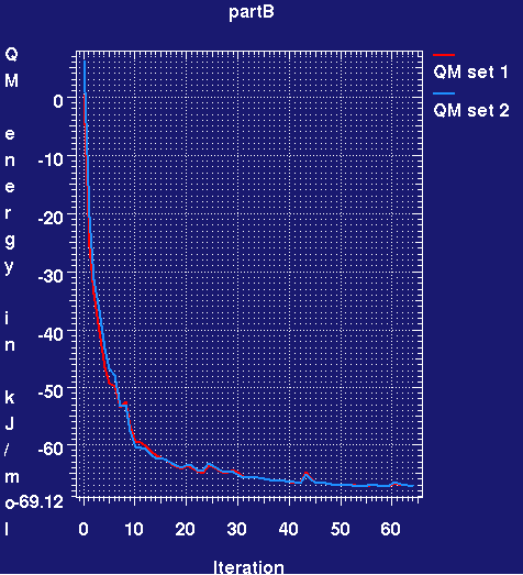
- The QM energy plotted is relative to the initial energy for the first set. It can be seen that during refinement the RM1 energy for both ligands rapidly drops and then plateaus. What does this mean? Basically because in the PDB deposition the IOG ligand has been refined using CNS restraints, the ideal geometry is slightly different. All that is happening is that the ligand is adjusting its conformation to that preferred by RM1. The adjustments are small.
- While the job is running, graph_autobuster_R can be used to monitor the progress of Rwork and Rfree:
graph_autobuster_R -d partB -launch
- In addition, after one big cycle is completed the refined structure and its maps can be quickly examined with:
visualise-geometry-coot partB
- Once partB has completed examine the IOG ligand geometry.
visualise-geometry-COOT partB
- In COOT also load 2i0g.pdb for comparison.
- Use COOT "Go to atom" to find IOG A 1.
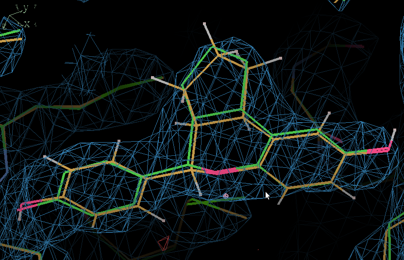
- Here the QM-refined ligand is shown in orange, and compared with the original PDB conformation in green. The 2Fo - Fc density is contoured at 1.3 RMSD and the difference density at 3 RMSD.
- In terms of fitting the macromolecular data the changes are small and the fit to the map is the same.
- However, if you use Mogul to examine the bond lengths and angles for the QM-refined I0G in comparison to the original I0G from the PDB file, many fewer deviations are found (see analysis below).
- Looking at the Rwork/Rfree graph for the completed partB job, the refinement produces an nice drop in Rfree by about 1.2%. Is this due to the use of QM for the ligand? Of course it isn't! - the difference is the result of running a long refinement with BUSTER, particularly with -autoncs. We will show this by running a control refinement in part (C).
- Advanced users You will notice that both Rwork and Rfree are still dropping at the end of the partB refinement. We also have not applied TLS. To get the most out of the model before additional building it is appropriate to do a further autoBUSTER refine run. Notice that this still uses -qm I0G but this time with -M TLSbasic as well as -autoncs.
  time refine                 \
  -p partB/refine.pdb         \
  -m 2i0g.mtz                 \
  -autoncs                    \
  -l I0G.grade_PDB_ligand.cif \
  -qm I0G                     \
  -M TLSbasic                 \
  -d partB2 > partB2.log      &
- The further partB2 refinement with TLS results in a drop of Rwork/Rfree from 0.2153/0.2517 to 0.2053/0.2420 and further improvement in MolProbity scores. To keep things simple we will use the original run.
(C) Control refine with dictionary -l I0G.grade_PDB_ligand.cif
- As a control do the same refine job but leave out the -qm so I0G geometry will be handled by the GRADE dictionary:
time refine                 \
-p 2i0g_addhI0G.pdb         \
-m 2i0g.mtz                 \
-autoncs                    \
-l I0G.grade_PDB_ligand.cif \
-d partC > partC.log &
(D) Analysis comparing the QM and dictionary refine jobs
- Let's compare results, first concentrating on the overall refinement metrics:
- refine.log reported CPU time on a Intel(R) Core(TM)2 CPU 6700 @ 2.66GHz (4 year old basic workstation)
- BUSTER values
Let's now look at the I0G ligand, concentrating on the A site (because the B site is really pretty much identical). First let's extract the A site ligand from the various coordinate files (together with the CRYST1 card so the resultant PDB file works with crystallographic tools).
egrep "CRYST1|I0G A" 2i0g.pdb > 2i0g.I0G_A.pdb
egrep "CRYST1|I0G A" partB/refine.pdb > partB.I0G_A.pdb
egrep "CRYST1|I0G A" partC/refine.pdb > partC.I0G_A.pdb
We can assess how well the different ligand conformations fit to the density by eye using COOT with the result that they appear very similar and fit the density about equally well. A correlation coefficient to the BUSTER 2Fo-Fc map can be found by running:
corr -p partC.I0G_A.pdb -m partB/refine.mtz
These confirm that the density fits are equally good.
What about the geometry of the ligand? This can be assessed by the CCDC Mogul program, compared to similar CSD structures. We have found that a useful metric is obtained by running Mogul in default mode and searching for "All fragments", "All bond fragments", sorting by Z and finding the number of bonds with Z above 2, as well as the average Z score (using a spreadsheet such as OpenOffice or gnumeric).
- So both the refinement using QM (RM1 method) for I0G and that using a GRADE dictionary improve the "geometric quality", as assessed using Mogul compared to the original PDB model. As GRADE uses Mogul data to derive many of its restraints the average Z-score value is lower for GRADE.
- From these results we can conclude:
- Using QM with the RM1 method only marginally slows a BUSTER refinement.
- That both refinements show good improvements over the PDB entry,
- and that looking at either the partB or partC maps shows that quite a bit of density for ordered solvent has appeared in particular next to atom O20 of the ligand.
- Although the Rfree is marginally higher in the QM run, the differences are small and likely to be due to slightly different X-ray weight adjustment. In terms of the protein structure the two refinements are in essence identical (for instance compared to the effect of using TLS).
- So the exact restraint method used for the ligand does not effect the protein refinement - as really would be expected.
- That both QM (RM1) and refinement with a GRADE dictionary produce good ligand geometry as assessed by Mogul.
(E) Assessing ligand strain energy and motions for the QM result
- In part (B) we saw how it is possible to monitor the QM energy for the ligand during a refinement relative to its initial position. However, what we really want to assess is the strain energy of the ligand. To do this we want to find what the quantum energy of the ligand in its refined position is with respect to the minimum energy conformation of the ligand. Normally this can be found by doing a "geometry optimization" of the ligand in isolation from its position in the refined complex.
- First extract the ligand coordinates for the A site. This can be done with an editor or using the egrep command. N.B.: BUSTER requires that all PDB files have a CRYST1 line:
egrep "I0G A|CRYST1" partB/refine.pdb > partB.IOGA.pdb
- Then use gelly_refine to geometry optimize the ligand:
gelly_refine -p partB.IOGA.pdb \
    -l I0G.grade_PDB_ligand.cif -qm I0G \
   -d partE -o partE_out.pdb \
   -max 1000 -glim 0.01 -jiggle_xyz 0.01 > partE.log &
- The run uses a dictionary and -qm IOG
- It also increases the default maximum number of steps and reduces the convergence limit: this is useful to ensure that a minimum is actually reached. The -jiggle_xyz 0.01 argument jiggles the input coordinates by a small amount: this is useful to ensure the optimizer does not get stuck in a saddle point.
- The command graph_autobuster_QM can be used to find the QM energy of the ligand in the optimization.
graph_autobuster_QM -d partE
...
# final raw QM energies   =   -405.27 kJ/mol
- So relaxation drops the QM energy to -405.27 kJ/mol. This energy can be used as a reference point to find the strain energies for the partB result:
graph_autobuster_QM -d partB -qmzero -405.27
...
# final raw QM energies   =   -399.62  -399.61 kJ/mol
# -qmzero specified so report QM energies relative to -405.27
#     big   small   iters      QMener_01      QMener_02
#       5      33     346           5.65           5.66
- So the strain energy of bound ligand is 6 kJ/mol relative to the isolated geometry-optimized form.
- The optimized coordinates for the ligand partE_out.pdb (purple) can be compared to the refined ligand (orange) using COOT:
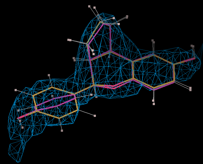
- It can be seen the relaxation is principally a rotation of the phenyl ring. The 2Fo-Fc density in the refined protein defines the orientation of the ring. Relaxation of the ring would cause it to have a short contact with Leu 339.
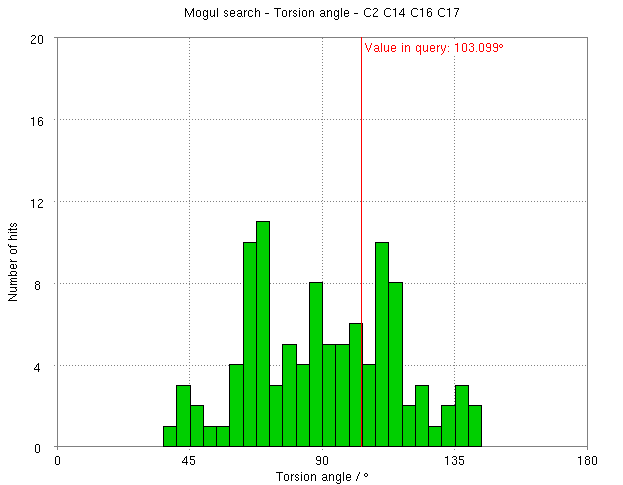
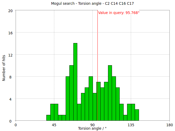
- The torsion angle C2-C14-C16-C17 measures the rotation of the phenyl ring. This torsion angle changes from -148.82 degs. (partB) to -103.10 degs.
- It is interesting to compare these results with the Mogul distribution of similar torsion angles from CSD small molecule structures. In the refined structure the ligand phenyl torsion angle would be regarded as "unusual" on the edge of the expected torsion angle from related CSD structures :
- But relaxation with RM1 allows shifts the torsion angle into the range to be expected for small molecule structures.
- The relaxation relieves short contacts between the phenyl ring and rest of the structure.
Page by Oliver Smart and Ian Tickle from 14 Feb 2011, modified November 2013. Any questions regarding our software or this wiki should be directed to buster-develop@globalphasing.com
