Content:
1VJO - SAD
The Se-MET data was collected at the Se-peak. A Fluorescence scan gave f'/f" values of
| Dataset | Wavelength | f' | f" |
| peak | 0.979 | -5 | 5 |
The sequence (393 residues) contains 9 methionines - 1vjo.pir:
MGSDKIHHHH HHMAQIISIN DNQRLQLEPL EVPSRLLLGP GPSNAHPSVL
QAMNVSPVGH LDPAFLALMD EIQSLLRYVW QTENPLTIAV SGTGTAAMEA
TIANAVEPGD VVLIGVAGYF GNRLVDMAGR YGADVRTISK PWGEVFSLEE
LRTALETHRP AILALVHAET STGARQPLEG VGELCREFGT LLLVDTVTSL
GGVPIFLDAW GVDLAYSCSQ KGLGCSPGAS PFTMSSRAIE KLQRRRTKVA
NWYLDMNLLG KYWGSERVYH HTAPINLYYA LREALRLIAQ EGLANCWQRH
QKNVEYLWER LEDIGLSLHV EKEYRLPTLT TVCIPDGVDG KAVARRLLNE
HNIEVGGGLG ELAGKVWRVG LMGFNSRKES VDQLIPALEQ VLR
Data was processed with autoPROC, resulting in the file:
- 1vjo_01_scala.sca (peak)
1. Running autoSHARP
It is always best to start a new project by running the fully automated autoSHARP pipeline (Vonrhein, C., Blanc, E., Roversi, P. & Bricogne, G. (2007). Automated structure solution with autoSHARP. Methods Mol Biol 364, 215-30). From the results it is easily possible to run follow-up calculations to fine tune the heavy-atom model in SHARP, change density modification parameters, add additional datasets or include an existing partial model.
1.1. Files:
- copy the reflection file and the sequence file (monomer!) into your sharpfiles/datafiles directory
1.2. Starting autoSHARP:
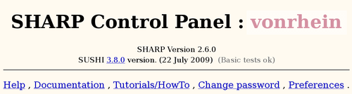
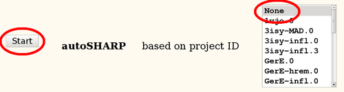
- from the main SHARP Control Panel (e.g. http://localhost:8080):
- Start autoSHARP based on None
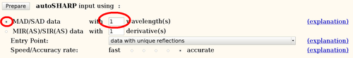
1.3. Define experiment type:
- on the following first page:
- specify to run MAD with 1 wavelengths
- leave the Speed/Accuracy level at the default (accurate)
1.4. Describe data and project:
- on the next page, fill out the following boxes or select appropriate items in pull-down menus:
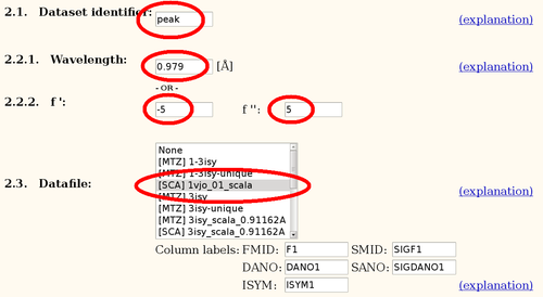
- in the General section: Project identifier (e.g. "1vjo"), Sequence file and No of expected sites
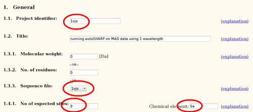
- for each Wavelength: Dataset identifier (e.g. "peak"), Wavelength, f'/f" (see above) and select the correct Datafile (since these are *.sca files, the column names can be ignored)
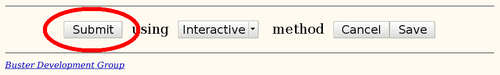
1.5. Run job:
- hit the Submit button
- go to logfile
autoSHARP_1vjo_07_500.png (file not found)
2. Interpreting autoSHARP output
The main autoSHARP logfile is a simple HTML document:
- The running job will append to it, so from time to time hit the 'reload' button on your browser (or "Ctrl-R").
- It only contains the most important information: more details are available by following the various links.
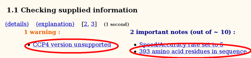
- There are notes, warnings and (hopefully not) errors. Warning messages are definitely worth a closer look. The notes will usually also contain important information about the datasets and/or progress of structure solution.
2.1. Input and data analysis:
Some warnings might be unavoidable, a typical example is the warning about a (potentially) unsupported CCP4 version. Since a specific SHARP/autoSHARP release was tested against the CCP4 version available at the time, autoSHARP will inform the user if a newer version is actually used during the run. However, it is very unlikely that this would have a significant effect upon the results if it is only an updated patch release of CCP4 (e.g. 6.1.13 when 6.1.1 was current at the time of the SHARP/autoSHARP release).
Each of those notes/warnings are hyperlinks to the details page where some additional information and/or explanation (usually as a link to the online manual) can be found.
Several notes towards the beginning of an autoSHARP job seem rather dull and trivial (like the number of residues). Nevertheless, those are good indicators that simple things like file format conversions have been done correctly (e.g. creating the PIR-formatted sequence file).
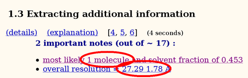
An analysis of asymmetric unit content (using Matthews coefficient) will show the most likely number of molecules given the monomer sequence. It is important that the sequence and the number of expected heavy atom sites are in sync: autoSHARP will multiply both the sequence and the number of sites to search for based on this analysis. Therefore, in most cases the monomer sequence and the number of expected sites per monomer should be given.
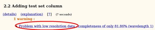
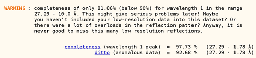
A warning about low completeness (in the lowest resolution shell) is often caused by either a very large beamstop shadow or a large number of overloaded reflections (and the lack of a low-resolution pass to measure those strongest reflections too). When following the hyperlink to the detailed information, autoSHARP tries to give easy to understand explanations to help the user:
2.2. Heavy atom detection:
Experimental phasing using a heavy atom model is obviously only possible if one can find this heavy atom substructure. As a general rule, one often needs much better heavy atom signal to find the sites in the first place, than is needed for phasing and solving the structure once a correct set of positions is available. For that reason, two distinct steps are required at this point:
- determining to what resolution a likely heavy atom signal is present
- being confident about a found heavy atom substructure solution
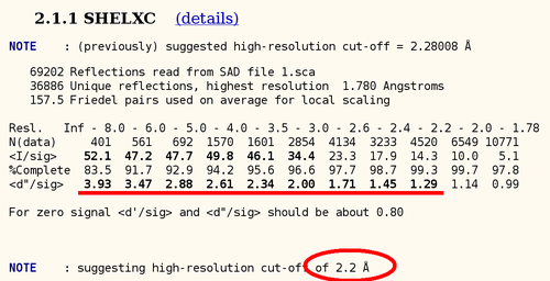
In the case of a SAD dataset, not a lot of statistics can be used to determine the high-resolution cut up to which a good heavy atom signal is available. One of those statistics is the anomalous difference over its sigma: here we can see that there seems to be good anomalous signal to about 2.2A (statistics from SHELXC), so this is a very good heavy atom signal:
autoSHARP uses this statistic to automatically cut the resolution used in heavy atom detection. The currently best trial solution from SHELXD is shown:
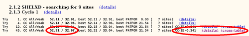
For this Se-MET experiment one would assume that all Se sites are fully occupied (with some caveat: N-terminal Met could be disordered, other Met could have alternate conformations or the Se-MET incorporation wasn't complete). Therefore, the plot of found sites should show the number of expected sites with high occupancy, followed by a clear drop when wrong sites (noise) start to appear:
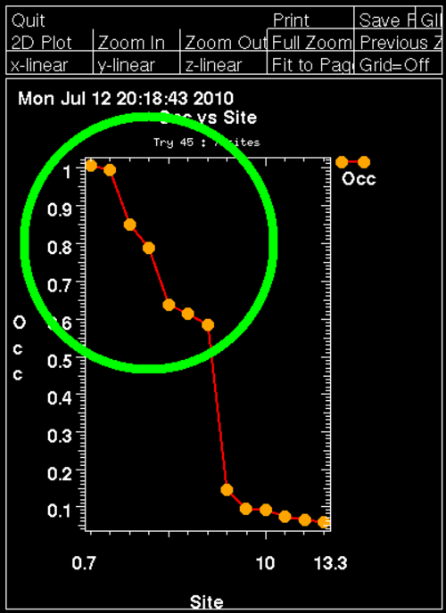
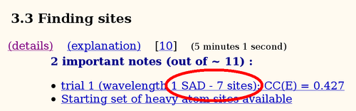
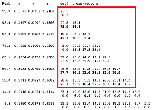
Here we can clearly see 7 mayor sites (out of 9 expected ones) - the N-terminal MET is probably disordered (the deposited PDB file has the first 16 residues missing, including 2 methionines). An additional confirmation of the found sites is the "crossword table" produced by SHELXD: it shows distance and peak height (Patterson symmetry minimum function) of self- and cross-peaks for the found sites in a Patterson map.
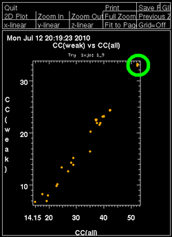
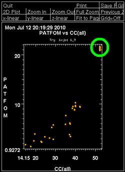
Once autoSHARP thinks that a reasonable solution has been found, additional statistics are provided as well as scatter plots for pairs of scores: CC(weak) vs CC(all) and PATFOM vs CC(all). The idea is that the substructure detection will lead a number of correct solutions as well as some wrong solutions - and that those two classes will be well separated in those quality scores. If these plots show no clear separation of clusters (or at least one solution significantly better than the majority), it is unlikely that the found substructure is actually correct - unless one has an extremely strong heavy atom signal and basically all solutions are correct.
It is important to have some confidence in the substructure solution, since otherwise the following steps can lead to a very large number of phase sets that will be difficult to judge and analyse.
2.3. Heavy atom refinement, phasing and model adjustment:
Once a set of heavy atom positions are found, their parameters (position, occupancy and B-factor) as well as scale and non-isomorphism parameters will be refined in SHARP. Ideally, all initial sites should have their parameters refined to meaningful values resulting in a set of good phases:
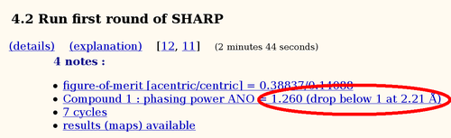
A very useful criteria to judge the quality of a set of phases is the resolution at which the phasing power drops below one. This should be a value similar to other criteria of heavy atom signal quality (correlation of anomalous differences or Rmeas/Rmeas0 comparison and correlation between half-sets as given in SCALA).
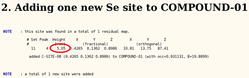
To adjust the current heavy atom model, the so-called "residual maps" (log-likelihood gradient maps) are analysed to e.g. detect wrong or additional sites. Here we get some indication of an additional site (remember, we only found 7 out of 9 sites so far), but the peak has a fairly small height:
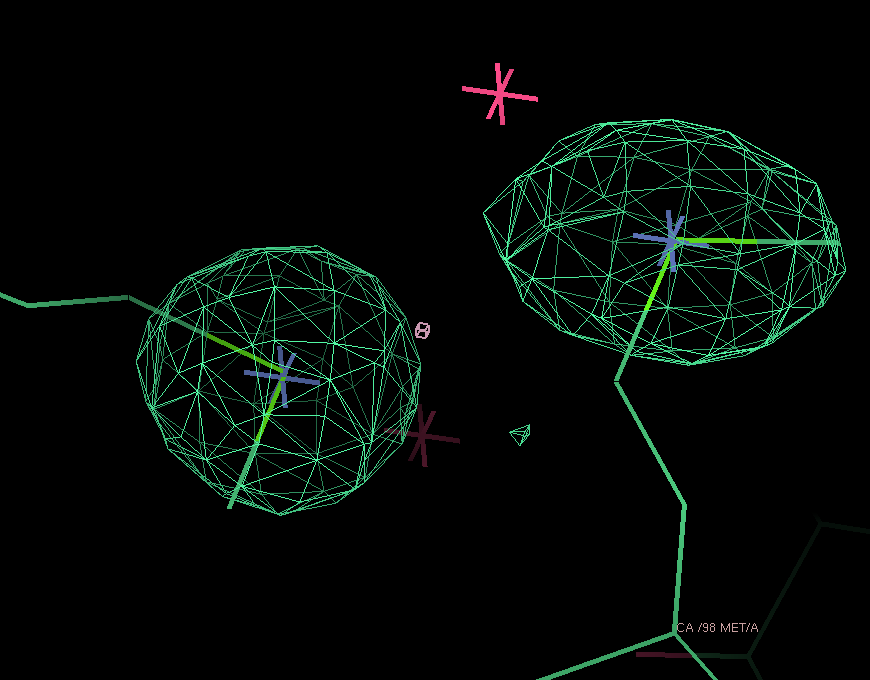
After adding this minor site (which isn't modelled as any atom in the deposited PDB file), the phase information improves only marginally. Visual inspection of the residual maps can show some typical features of methionines (or Se-MET heavy atom positions): alternate conformations of the side-chain, resulting in slightly split heavy atom sites:
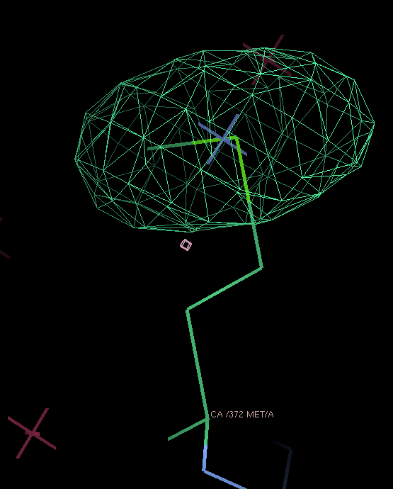
THose could be modeled as either split sites or heavy atoms with an anisotropic B-factor:
| Se-MET | Split site | Anisotropic B-factor |
| 98 | 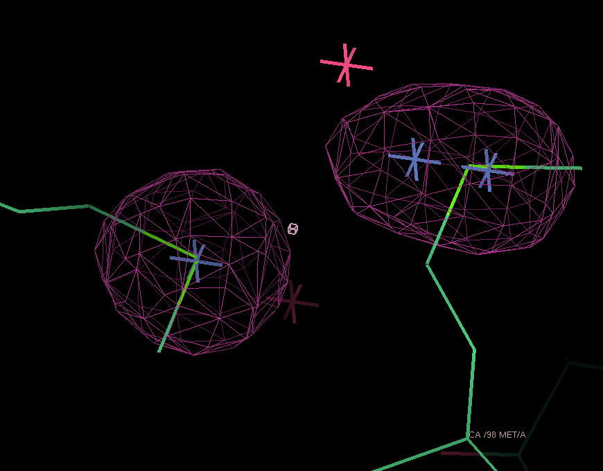 |
 |
| 372 | 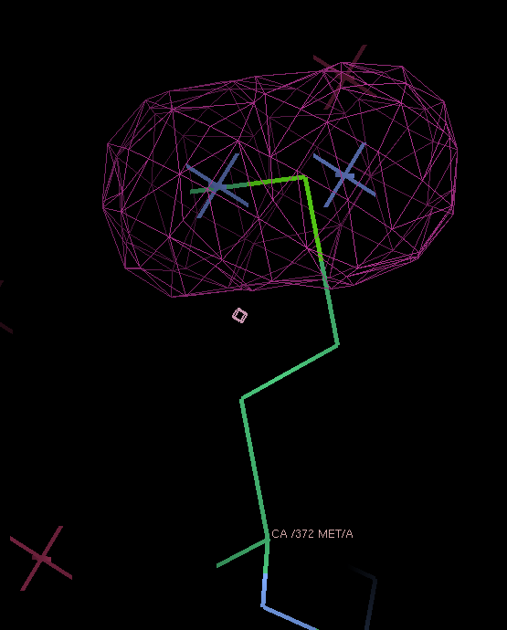 |
 |
2.5. Density modification:
Once a set of experimental phases is available, the decision about the correct handedness of the heavy atom substructure (and corresponding enantiomeric space group) needs to be made. In nearly all cases, the heavy atom solution would also be consistent with the data after inverting all heavy atom positions through the origin. For several spacegroup this would also result in a change to the enantiomorph (P41 to P43 etc). Important: there are only ever two possibilities to test since a change of substructure handedness automatically means a change to the enantiomeric space group.
The two phase sets should be easily distinguishable when calculating electron density maps: one should give a chemically sensible map whereas the other should be basically just noise. To distinguish those two cases, we use a single cycle of density modification to compare some statistics (which are combined into a 'score'):
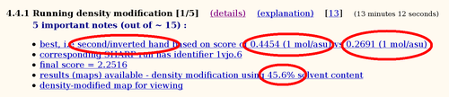
Here the inverted hand seems to give a better score than the original hand. Since space group C2221 doesn't have an enantiomorph, only the heavy atom positions need to be inverted (through the origin).
After deciding on the hand (and therefore phase set), these experimental phases are improved through standard density modification procedures using solvent flipping. A series of such runs is performed with varying values of solvent content to get the best map possible. Here the optimal solvent content (for creating a map with the best statistical indicators) is surprisingly close to the theoretical value calculated earlier. This is not necessarily always the case - but at this point we are mostly interested to know whether the structure has been solved or not.
2.6. Automated model building:
The hopefully best electron density map after density modification is used for automatic model building using ARP/wARP:
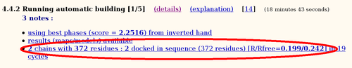
Of the expected 393 residues, 372 can be built into this map (the deposited PDB file contains 377 residues).
2.7. References and timing:
At the end of an autoSHARP run, some references for used software or methods are given. These could be used directly in any manuscript using results from SHARP/autoSHARP. There is also a little table summarizing the time spent in each step.
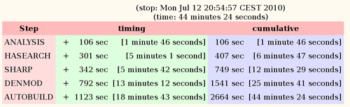
Most time is spent in the real-space calculations for density modification and model building towards the end. The timings here are for a Dell latitude D630 with Core2 Duo T7700 (2.40GHz).