| autoPROC Documentation |
previous |
next |
| Interpreting autoPROC output |
|
autoPROC Documentation : Interpreting autoPROC output
| Copyright |
© 2015-2018 by Global Phasing Limited |
| |
| |
All rights reserved. |
| |
| |
This software is proprietary to and embodies the confidential
technology of Global Phasing Limited (GPhL). Possession, use,
duplication or dissemination of the software is authorised only
pursuant to a valid written licence from GPhL.
|
|
| Documentation |
(2015-2018) Clemens Vonrhein, Claus Flensburg, Wlodek Paciorek & Gérard Bricogne |
| |
| Contact |
proc-develop@GlobalPhasing.com |
Contents
A typical sequence of data processing will consist of
- Preparation: defining sweeps and datasets,
checking and parsing of command-line arguments and (potentially)
giving initial warnings
- Spot search and indexing: finding spots and
attempting indexing - including tests for multiple lattices and
ice-rings
- Initial integration and space group
determination: if no known space group and cell was given,
determine most likely space group from initial integration
- Integration: integrate images of a given
sweep and perform parameter post-refinement
- Scaling, merging and analysis: internally scale the
integrated intensities (under space group symmetry), analyse
data for anisotropy (as well as for an adequate high-resolution limit) and create
merged reflection files in different formats
- Multi-sweep datasets: if multiple sweeps
(orientations, wavelengths, exposures etc) are present, combine
these and internally scale all of them together while merging
those with a common characteristics (usually: wavelength)
together;
The output of autoPROC is organised as a series of files and
directories, including plots (in PNG format - see here for how to view them) and scripts that can
be run by the user interactively.
The examples shown below are based mainly on standard output
(i.e. what is printed to the terminal or saved into a logfile). Often
it is easier to look at the "summary.html" file instead:
this follows the same sequence of steps with very similar messages and
explanations - but probably provides easier access to results and
plots.
Since all important information is currently given on standard output
(stdout), it is a very good idea to always save this into a file. This
can be done e.g. via
process ... -d 01 > 01.log 2>&1     # bash/zsh/ksh/sh
 - or -
process ... -d 01 >& 01.log         # csh/tcsh
 . or -
process ... -d 01 | tee 01.log      # any shell (but note the
                                      limitation on exit status
                                      when using the tee command)
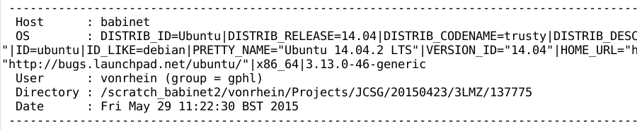
At the top of stdout will always be information about the machine,
account and date autoPROC was run (this can contain very long lines):
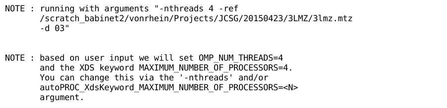
After checking for a syntactically correct command, the command-line
will be reported and additional information given:
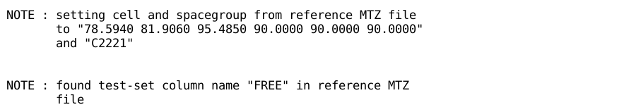
autoPROC will summarise what it understood from command-line arguments
and parameter settings, e.g. when giving a reference reflection (MTZ)
file:
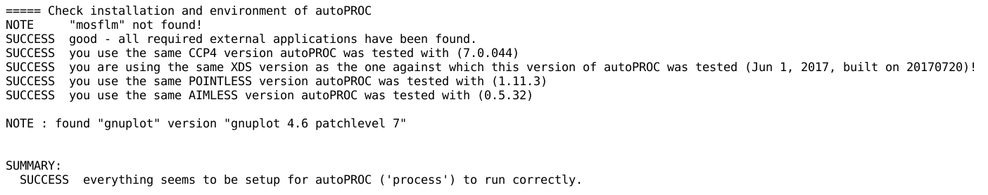
The program will test version information for external programs (like
XDS, POINTLESS or AIMLESS).
Please check the messages about external program versions given by
autoPROC carefully - if in doubt contact proc-develop@GlobalPhasing.com. You
should also check your autoPROC installation using
process -checkdeps
which should ideally report something like
Any warning or error message from the above step should be carefully
analysed.
BeamCentreFrom setting
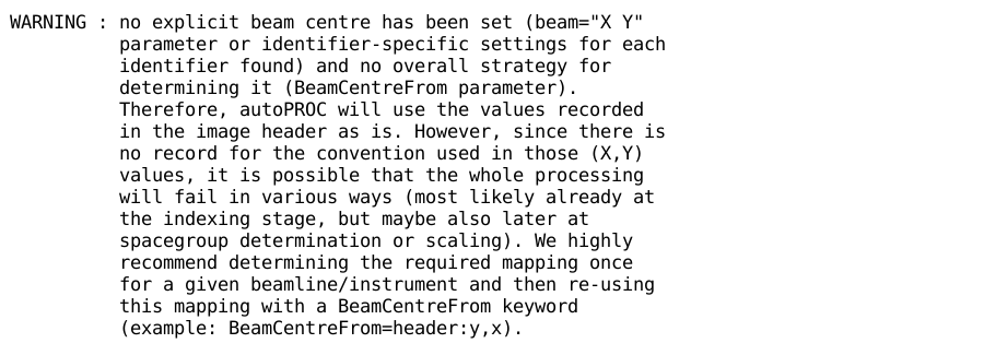
You will often get a warning about the beam centre coordinates:
Because the wrong specification of the direct beam coordinate is the
main reason for a failed indexing, this is stressed explicitly in that
message. You might want to also check the
autoPROC wiki for additional background information and a table of
relevant values for different beamlines and instruments.
Sweep/dataset definition
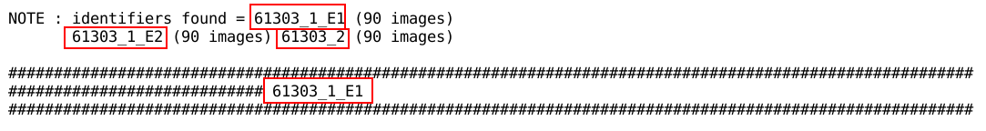
The last report in this section is a listing of identifiers and sweeps
found:
Make sure this is showing the (sweep) identifiers and number of images
as expected. There can be unexpected breaks if one or a few images are
missing. There could also be wrong concatenation of actually distinct
sweeps if the image files are named very similarly. In both these
cases it is advisable to use the -Id argument directly, e.g.
process -Id "test,/where/ever/images,test_####.cbf,1,900" ...
instead of relying on autoPROC (via the find_images tool) to
find sweeps or data automatically and correctly.
By default, autoPROC will search for spots on all images available and
gives those to indexing. autoPROC will try to optimise the initial
indexing solution for several reasons:
- getting the best starting point for subsequent integration
- detecting potential additional indexing solutions (split or
twinned crystals, cell increase due to radiation damage etc)
- obtaining a list of spots that can't be indexed at all and could
therefore be due to ice- or other powder rings, detector or
software errors (hot pixels, poor beamstop etc) or any other
possible problem during the experiment
Spots found per image (SPOT.XDS.SpotsPerImage.png)
We expect (or hope) to find a useful number of spots on all images
analysed - but there could be various reasons why this might not
always be true:
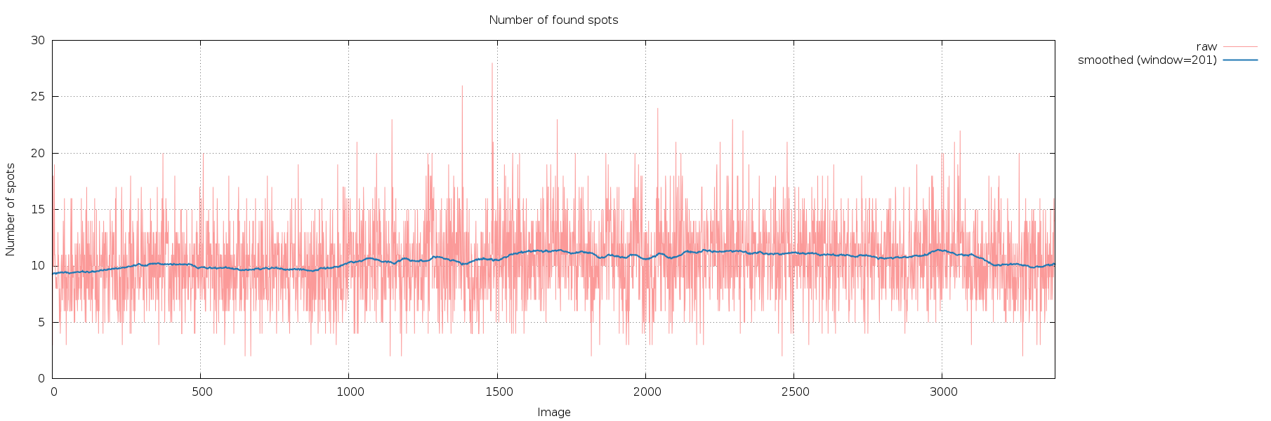
SPOT.XDS.SpotsPerImage.png
very similar number of spots found on all images
|
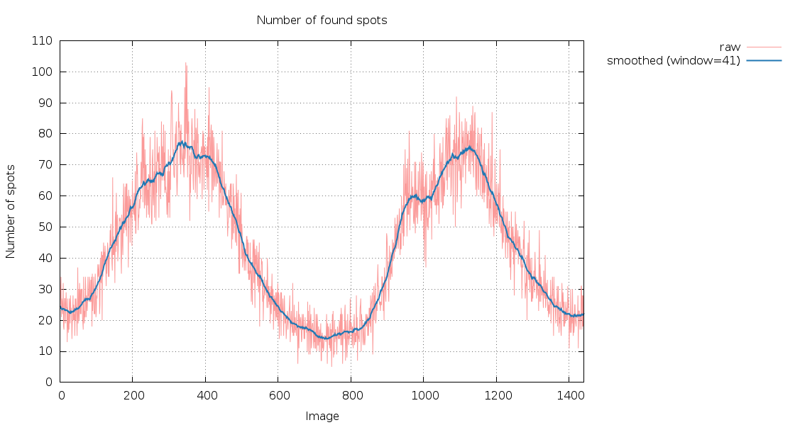
SPOT.XDS.SpotsPerImage.png
360 degree of data, showing a nice 180-degree periodicity (because
after half a rotation the beam should travel through the same part
of the crystal - just into the opposite direction): the difference
in number of spots could be due to anisotropy, significant
differences in cell dimensions, a split crystal (or non-merohedral
twinning) or because a second crystal moves in and out of the
beam. The important task is to look at the images (and predictions)
at the different maxima and minima of this graph, e.g. at image 340
and image 720.
|
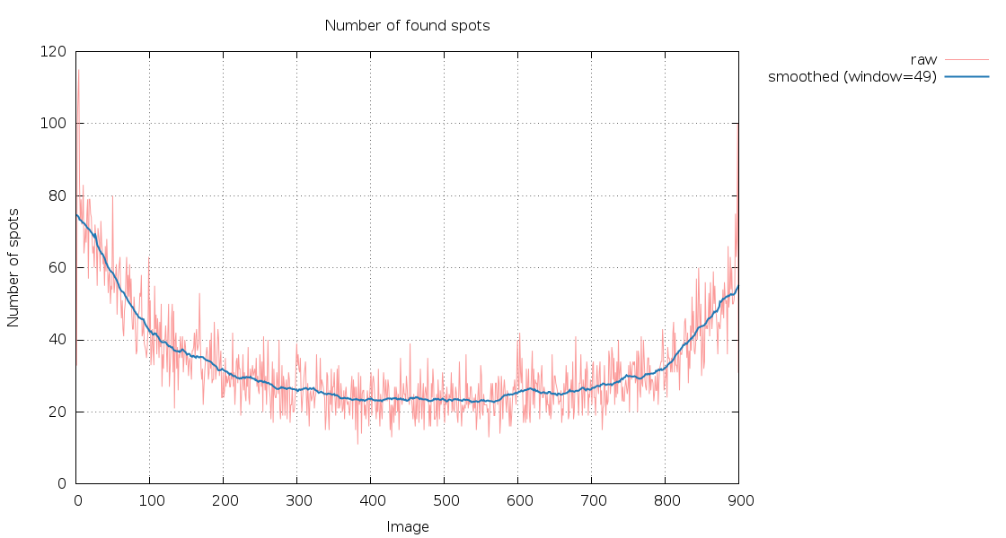
SPOT.XDS.SpotsPerImage.png
180 degree of data - the number of spots are nearly the same at
the first and last image (as expected): the small decrease might be
due to radiation damage.
|
| |
| |
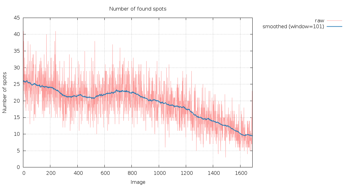
SPOT.XDS.SpotsPerImage.png
Only 167 degree of data, so difficult to interpret (we lack the
180/360 of data that allow a better check). The decrease in spot
numbers might be due to radiation damage.
|
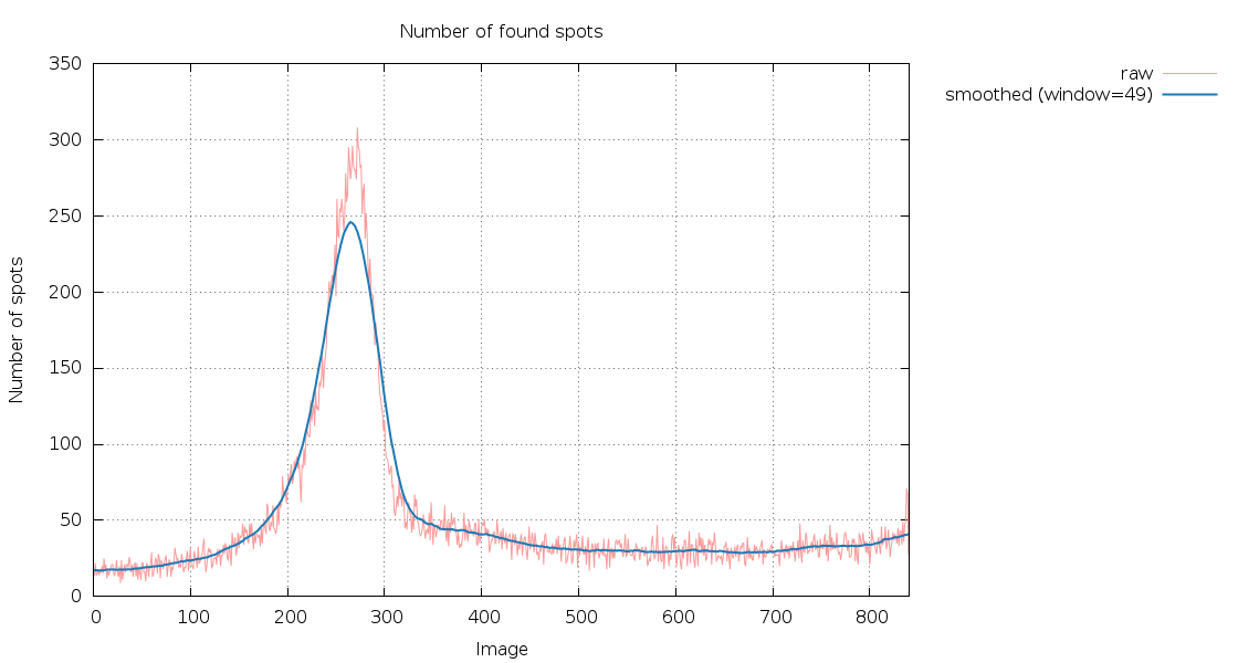
SPOT.XDS.SpotsPerImage.png
180 degree of data with a very distinct peak: either a very large
difference in cell dimensions, some extreme anisotropy or a second
crystal/lattice moving in and out of ht beam. Definitely
worthwhile checking images around 260.
|
|
Iterative indexing
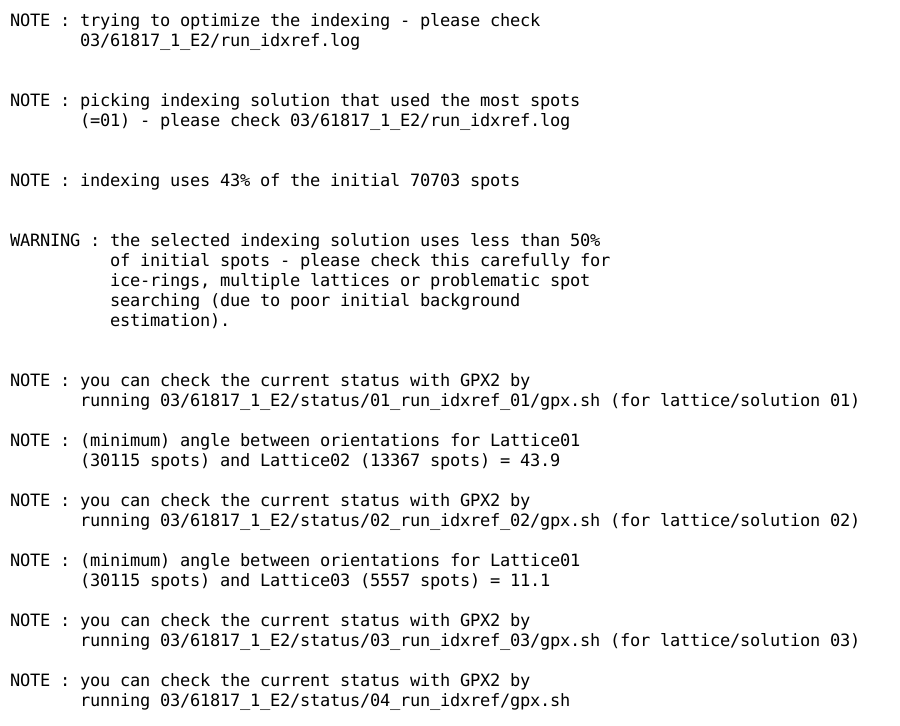
After this iterative indexing procedure, autoPROC will produce a
summary
and a plot (here 03/61817_1_E2/run_idxref_spot_hkl_hist.png)
showing the number of spots for each indexing solution as a function
of image number:
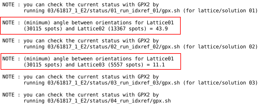
The (minimum) rotation between the different solutions is also
reported:
- small values might point to
- a slightly split crystal (depending on orientation of the
crystal this splitting might be visible on all images, but
often it is only detectable on a small range of images)
- a cell increase due to radiation damage (in which case the
later images have a significantly different set of cell dimensions
that can't be indexed satisfactorily with the earlier images -
resulting in two more or less exclusive indexing solutions with a
very similar orientation matrix)
- a large angular value could result from
- multiple crystals in the beam (dependent on mounting
system, ease of handling small crystals etc)
- a cracked crystal (long needles that broke into two parts
during mounting or handling)
- non-merohedral twinning (especially if the angle is
suspiciously close to 180, 120, 90 or such)
Proper interpretation of these results depends a lot on the actual
sample (keep a note and some screenshots of the crystal as it was
mounted during the experiment, ideally in several orientations),
previous experiments of the same crystal form (do you always get
multiple indexing solutions with the same relative angle between them)
and a very careful examination of the diffraction images together with
predictions.
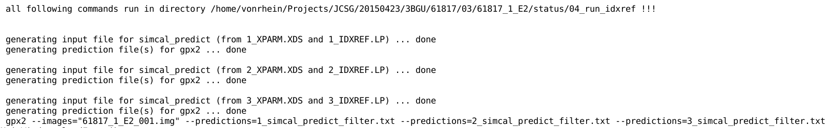
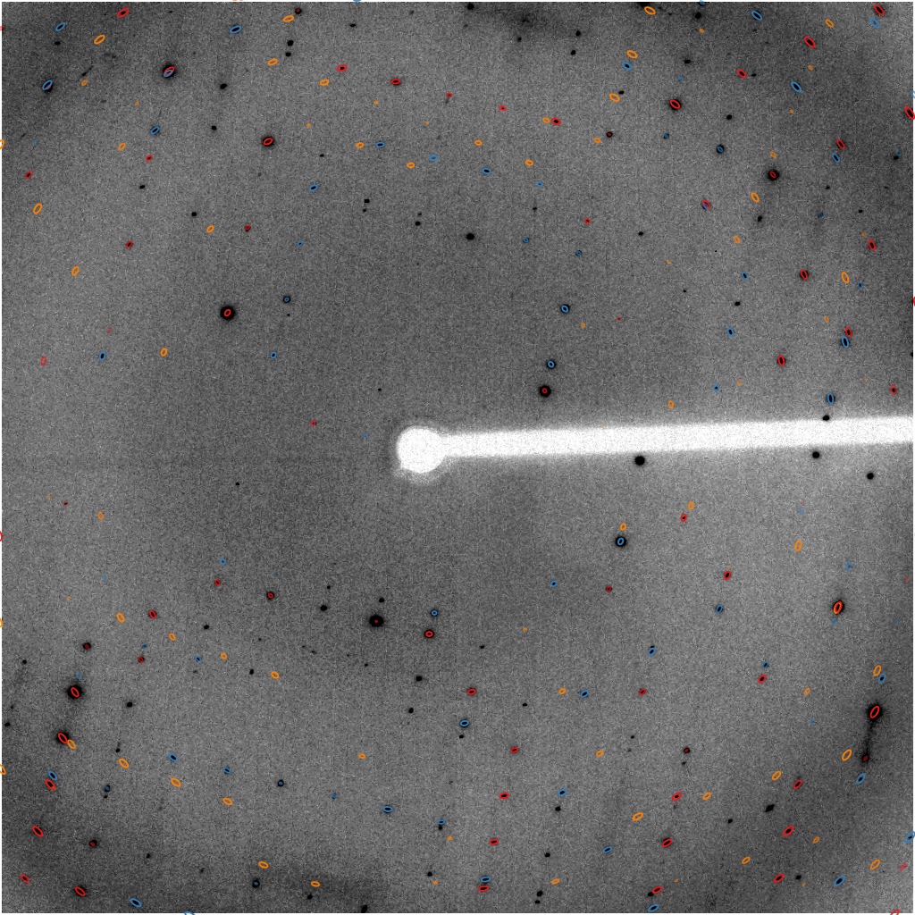
Visualisation with GPX2
Running for the above case the script for displaying predictions of
several indexing solutions
03/61817_1_E2/status/04_run_idxref/gpx.sh -lat 1,2,3
gives
and then shows predictions in GPX2:
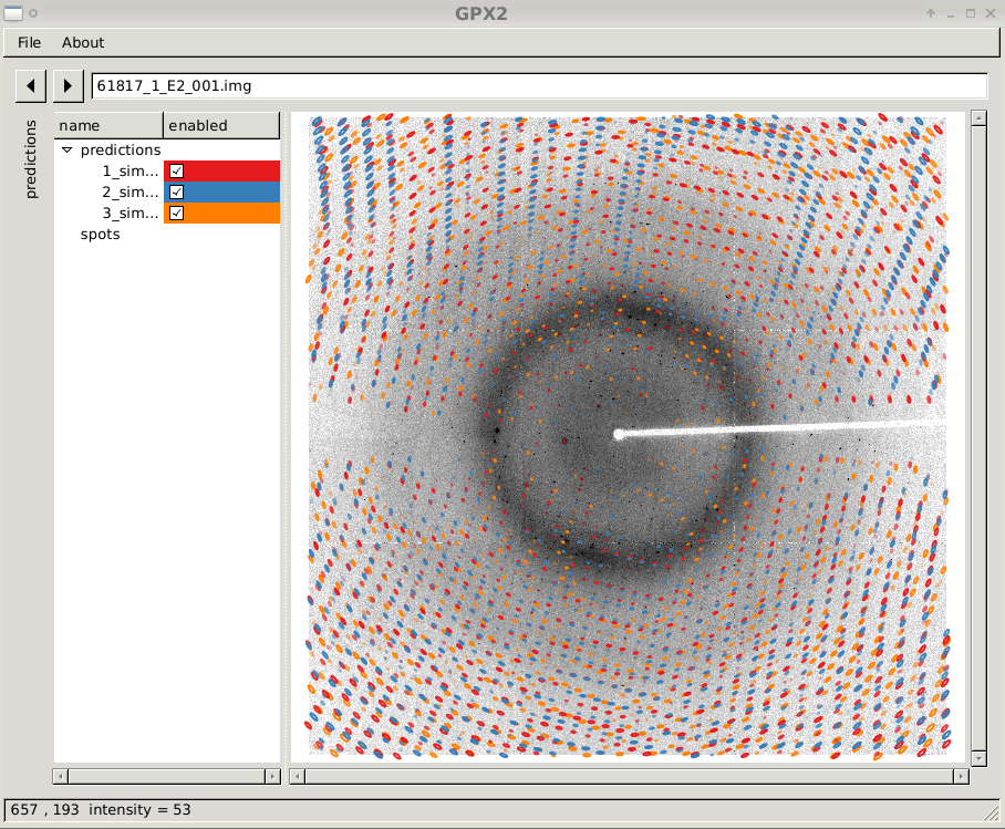
GPX2 showing three prediction sets
|
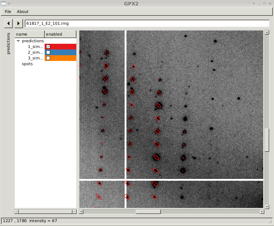
close-up of diffraction image with prediction sets 1
|
| |
| |
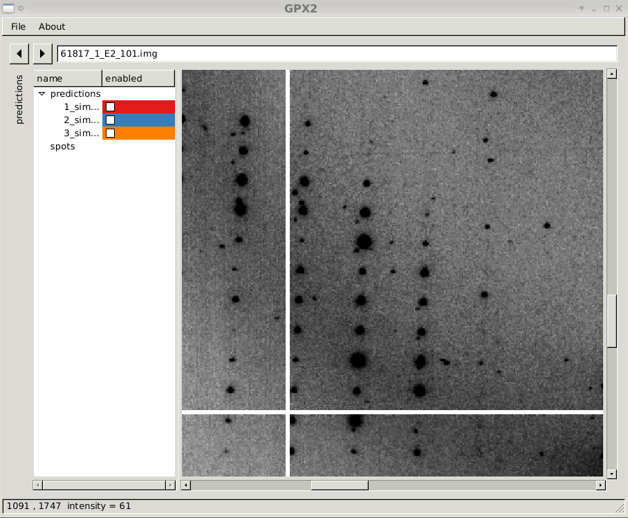
close-up of diffraction image
|
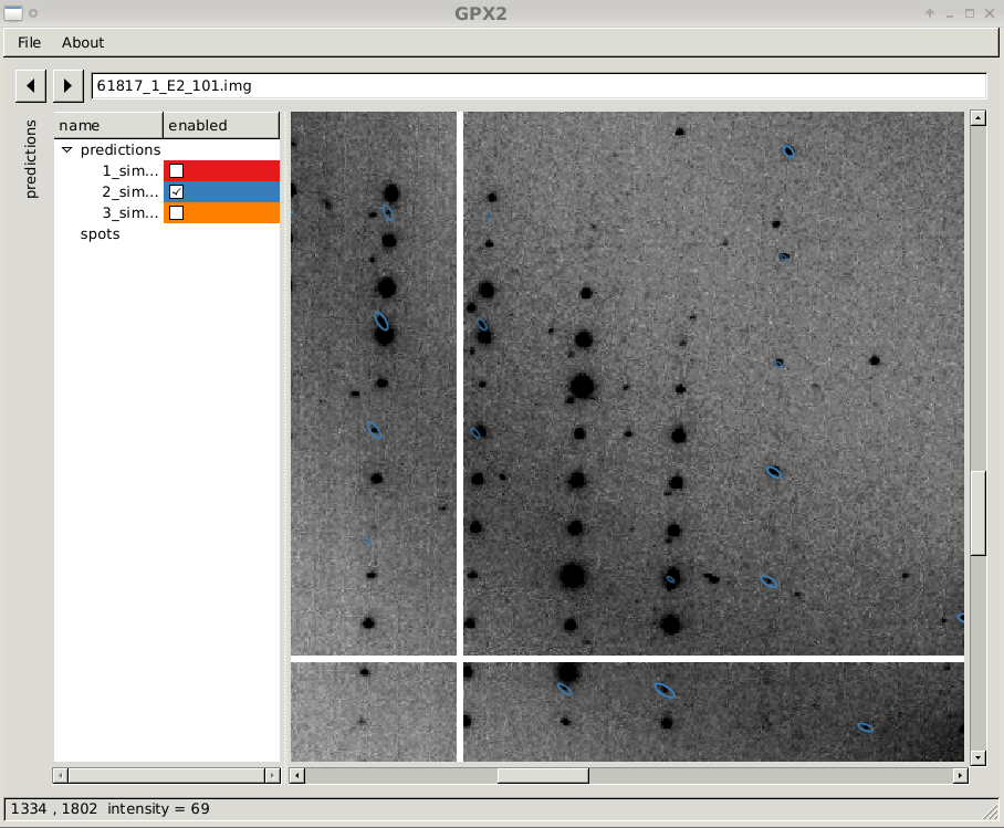
close-up of diffraction image with prediction sets 2
|
| |
| |
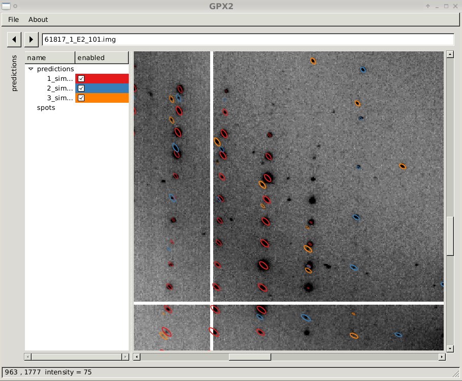
close-up of diffraction image with three prediction sets
|

close-up of diffraction image with prediction sets 3
|
Please note that this is using a default value for mosaicity which is
most likely not the correct one (and there could even be a different
mosaicity for each indexing solution, ie. lattice/crystal). In order
to re-run the same iterative indexing at the end of processing (of a
particular sweep), you could set the parameter autoPROC_ReRunIdxrefAtEnd=yes:
this will use the final set of parameters (for the indexing solution
used in integration).
By default, autoPROC will pick the indexing solution that uses the
most spots. If you want to make it pick another solution, set the
parameter XdsOptimizeIdxrefPickSolution
to the desired solution (as a two-digit number with leading zero) as
given on stdout, e.g. XdsOptimizeIdxrefPickSolution=02 would
pick solution number 02.
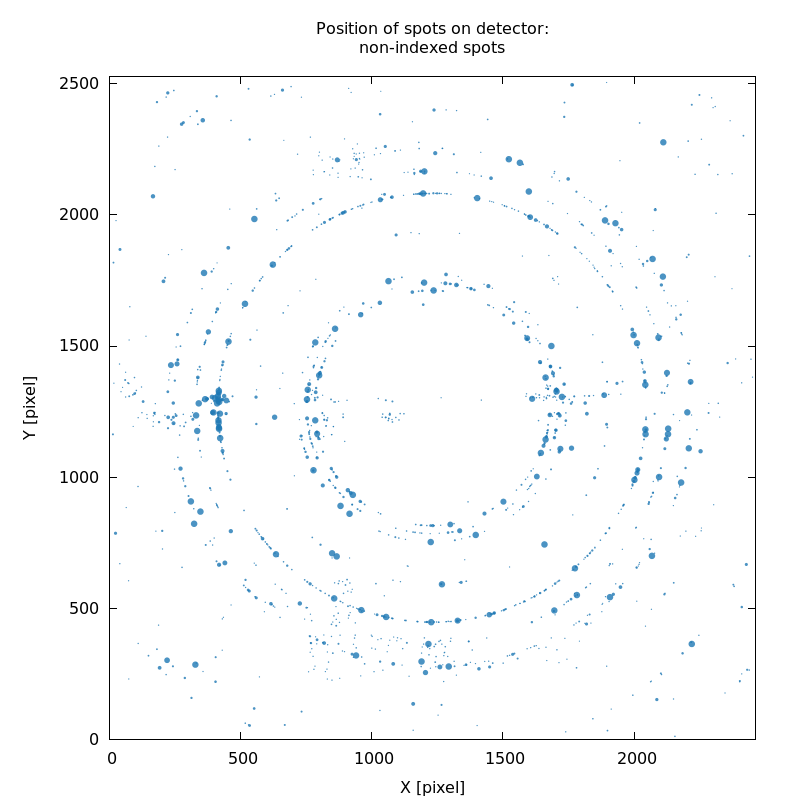
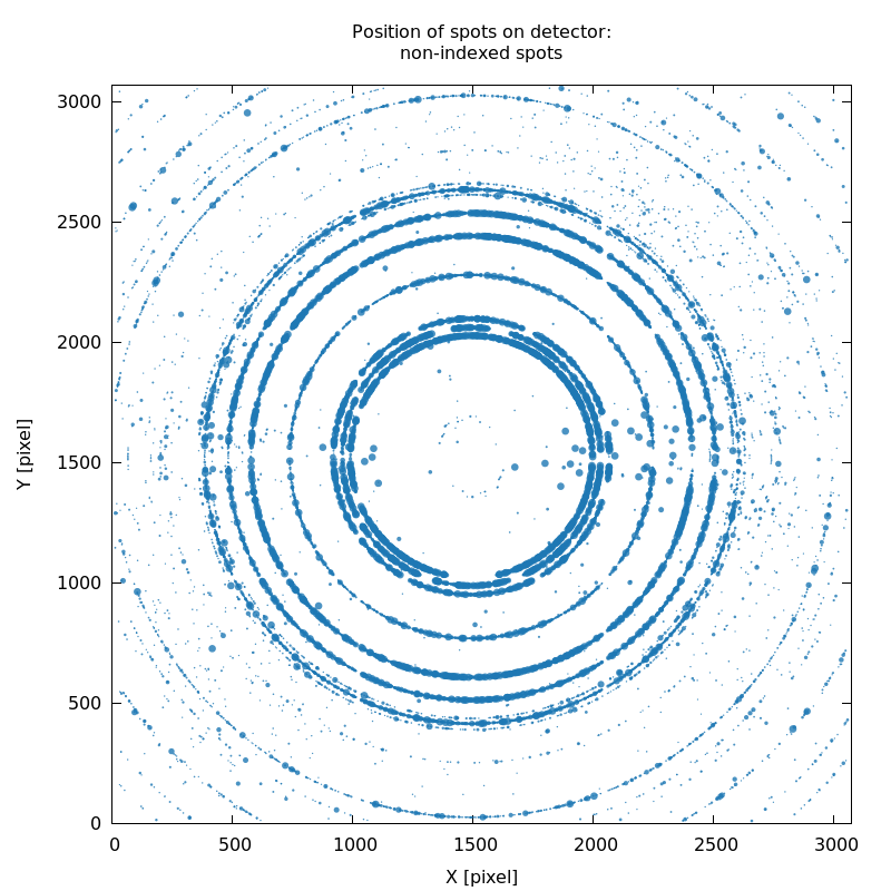
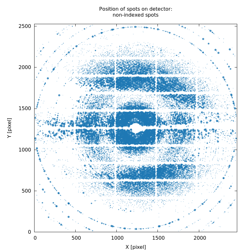
Unindexed spots (SPOT_never-indexed.noHKL.png)
A very useful plot shows the position (on the detector) of all spots
that could not be indexed by any of the trial solutions: SPOT_never-indexed.noHKL.png. It can show
ice-rings, detector calibration problems, missed lattices and more:
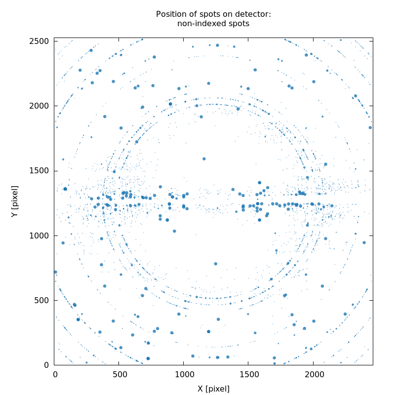
SPOT.noHKL.png
weak ice-rings
|
SPOT_never-indexed.noHKL.png
weak ice-rings
|
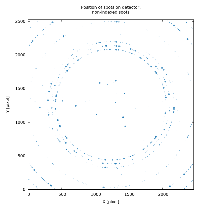
SPOT_never-indexed.noHKL.png
weak ice-rings
|
| |
| |
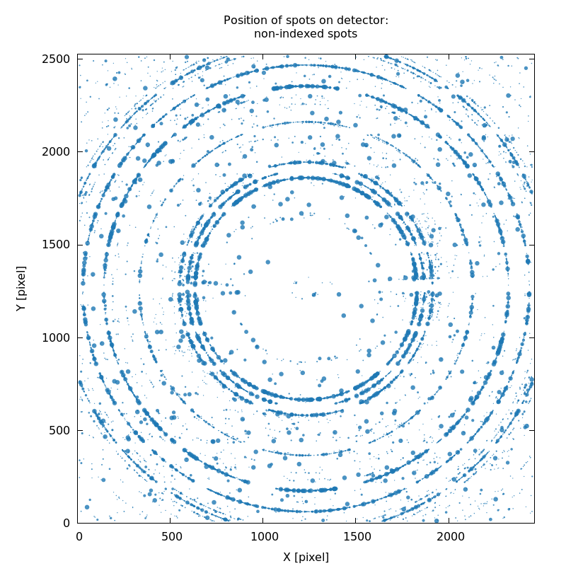
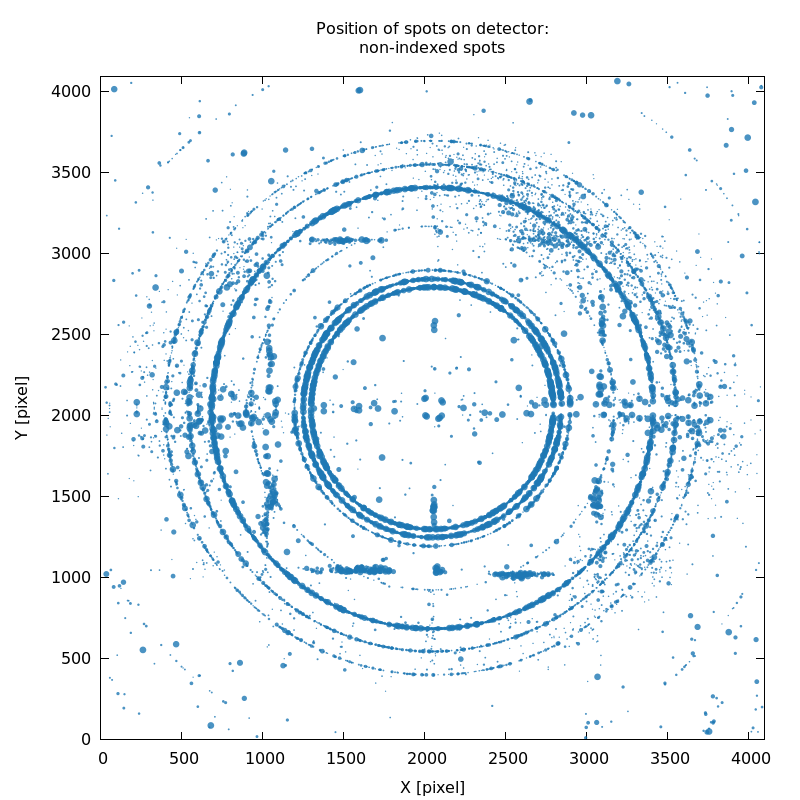
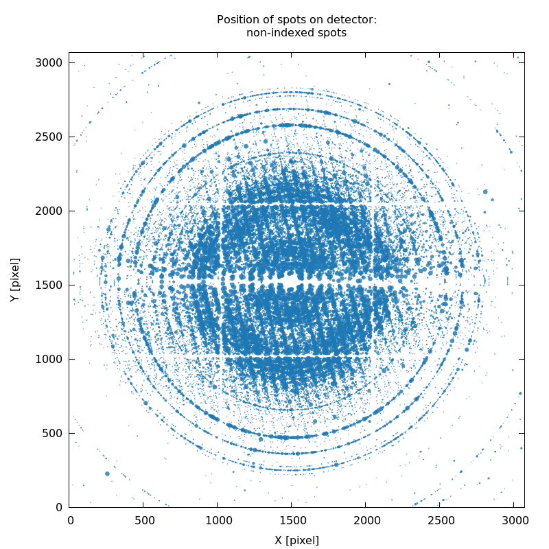
SPOT_never-indexed.noHKL.png
strong ice-rings
|
SPOT_never-indexed.noHKL.png
strong ice-rings
|
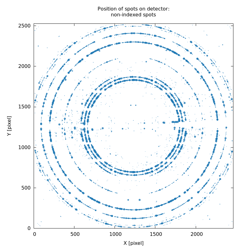
SPOT_never-indexed.noHKL.png
strong ice-rings
|
| |
| |
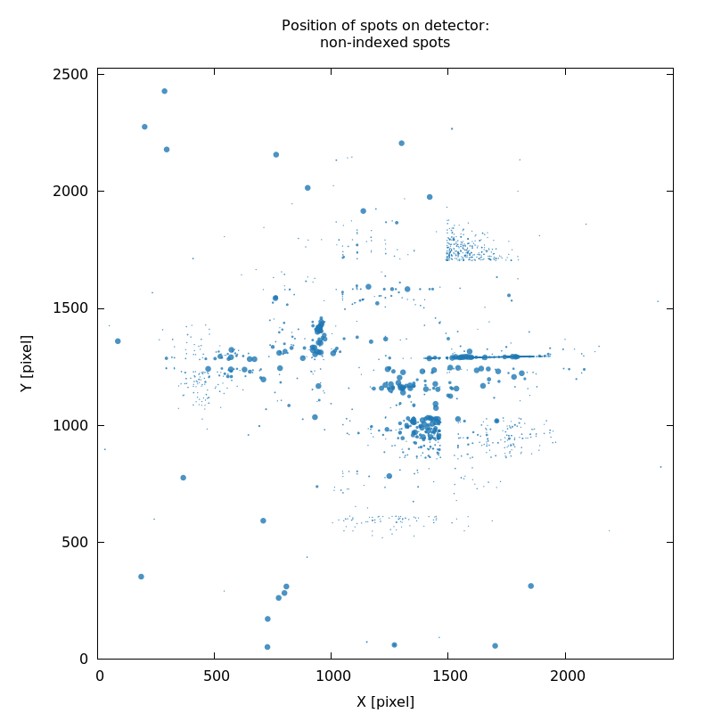
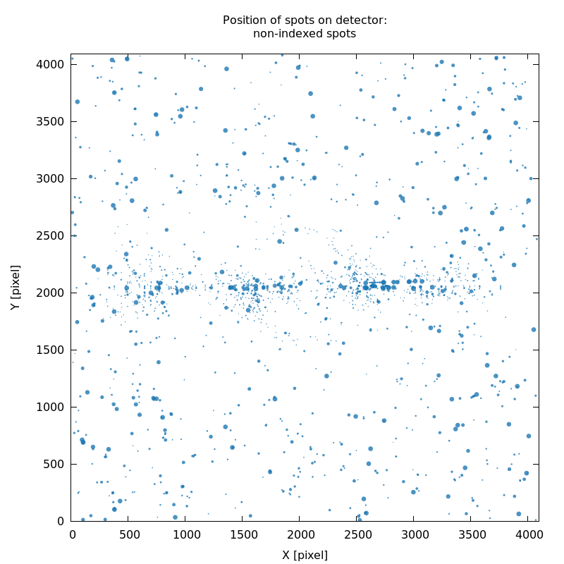
SPOT_never-indexed.noHKL.png
detector calibration
|
SPOT_never-indexed.noHKL.png
detector calibration
|
SPOT_never-indexed.noHKL.png
streaky/split spots
|
| |
| |
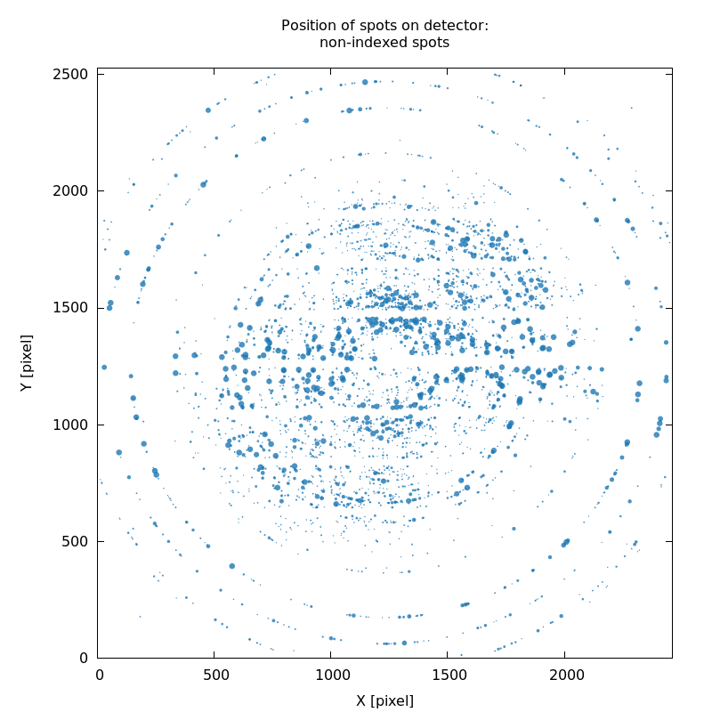
SPOT_never-indexed.noHKL.png
missed lattice(s), partly due to poor starting values describing
hardware geometry
|
SPOT_never-indexed.noHKL.png
missed lattice(s), partly due to poor starting values describing
hardware geometry
|
SPOT_never-indexed.noHKL.png
good - clean
|
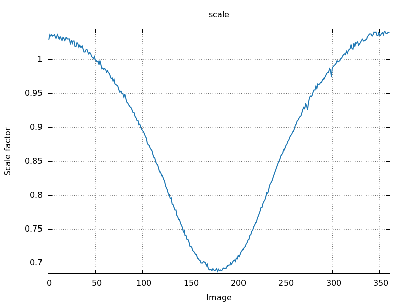
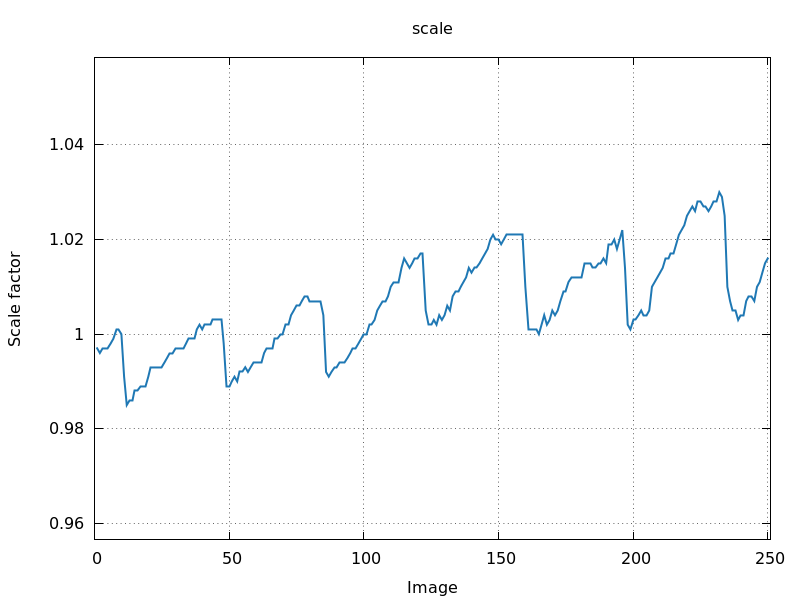
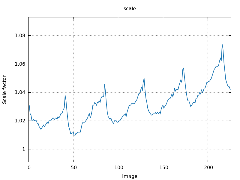
Image scale factor (scale.png)
A very useful plot is the per-image scale factor as a function of
image number (scale.png). Ideally we want to see a smoothly
varying curve that might show some periodicity (for 180- and
360-degree total rotation range):
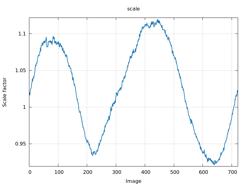
360 degree rotation
|
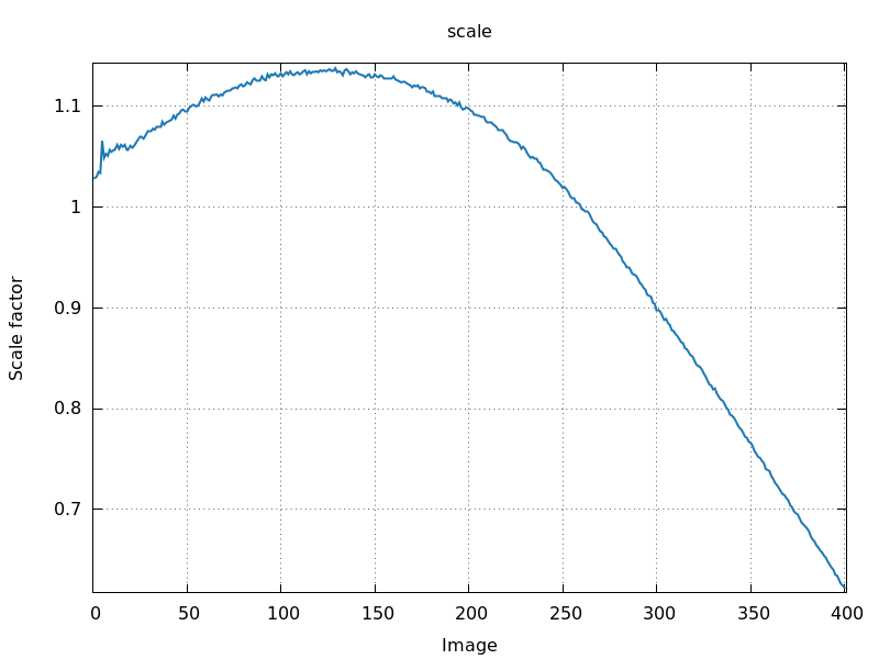
180 degree rotation
|
120 degree rotation
|
Sometimes there are single images that show an outlier value for image
scale:
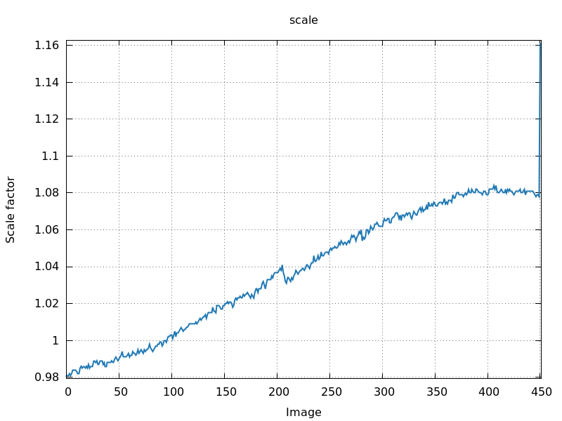
last image - shutter synchronisation
problem?
|
first image - shutter synchronisation
problem?
|
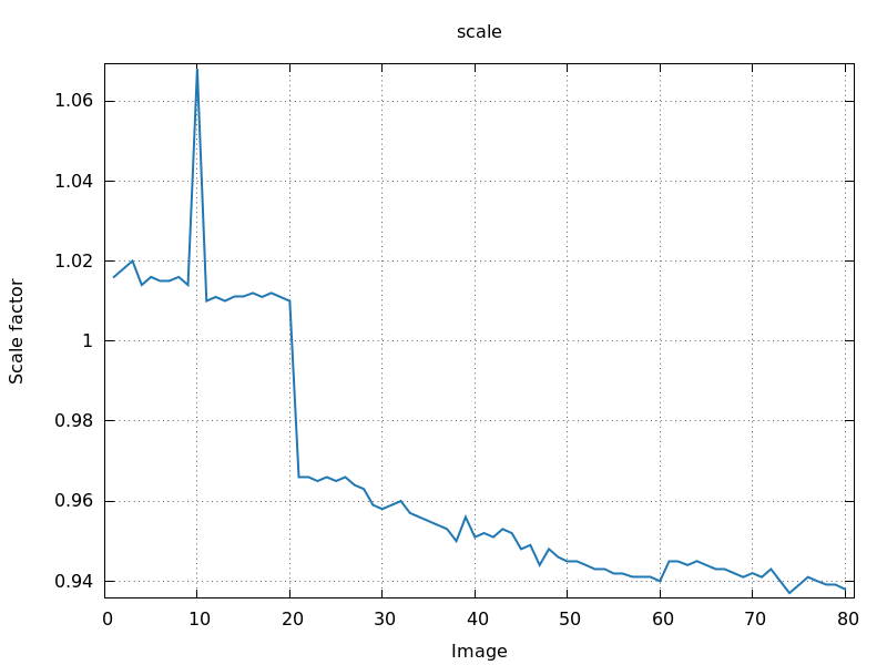
intermediate image - what could be
the problem?
|
If there are patterns visible that can't be explained by the
experiment (e.g. if some kind of inverleaving was done), this might
point back to beamline instrumentation issues (goniostat
instabilities, reproducibility or energy changes etc) or synchrotron specifics
(top-up modes, beam stability etc). In any case, such patterns should
be explainable (check with beamline staff and make them aware of those
plots) and ideally be avoided for future experiments.
0.25 degree per image
|
0.4 degree per image
|
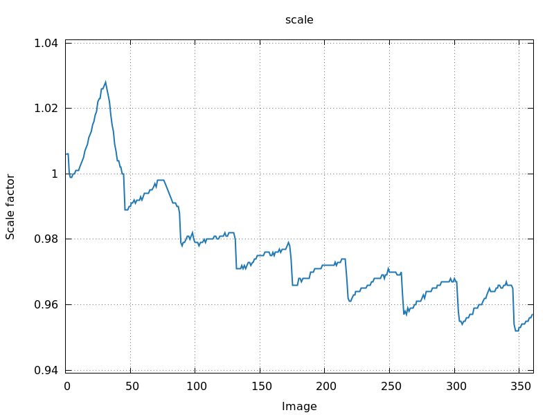
0.25 degree per image
|
Mosaicity and beam divergence (divergence-mosaicity.png)
During integration, XDS will by default determine crystal
mosaicity and beam
divergence directly from the diffraction images. The divergence-mosaicity.png plot
combines curves for beam divergence and mosaicity. However, this can
sometimes lead to poorer estimates at the beginning of the dataset -
which is why autoPROC will set those
parameters in subsequent integration steps (see also here):
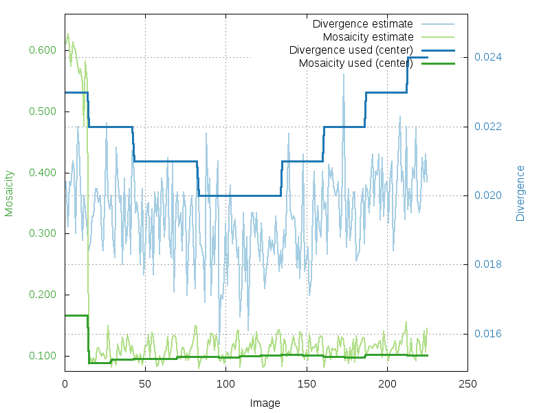
estimated (per image) and used (for central region) values of
mosaicity and divergence (as determined by XDS automatically)
|
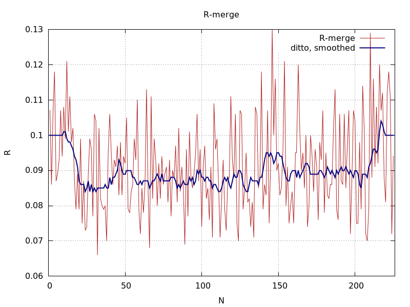
final Rmerge value showing poorer results for initial block of images
|
| |
| |
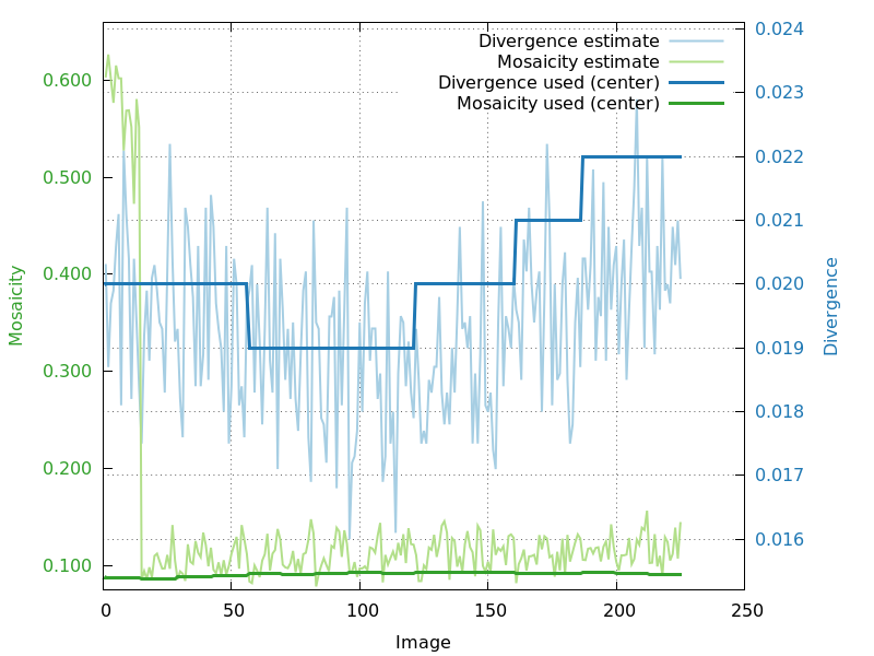
estimated (per image) and used (for central region) values of
mosaicity and divergence (when re-using overall values in
subsequent integration steps); this is the default in autoPROC
|
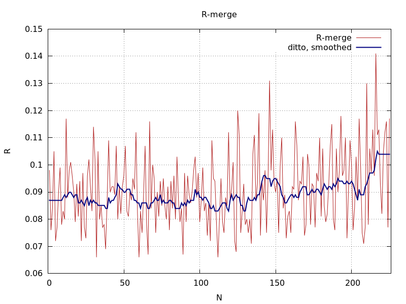
final Rmerge value showing better results also for initial block of images
|
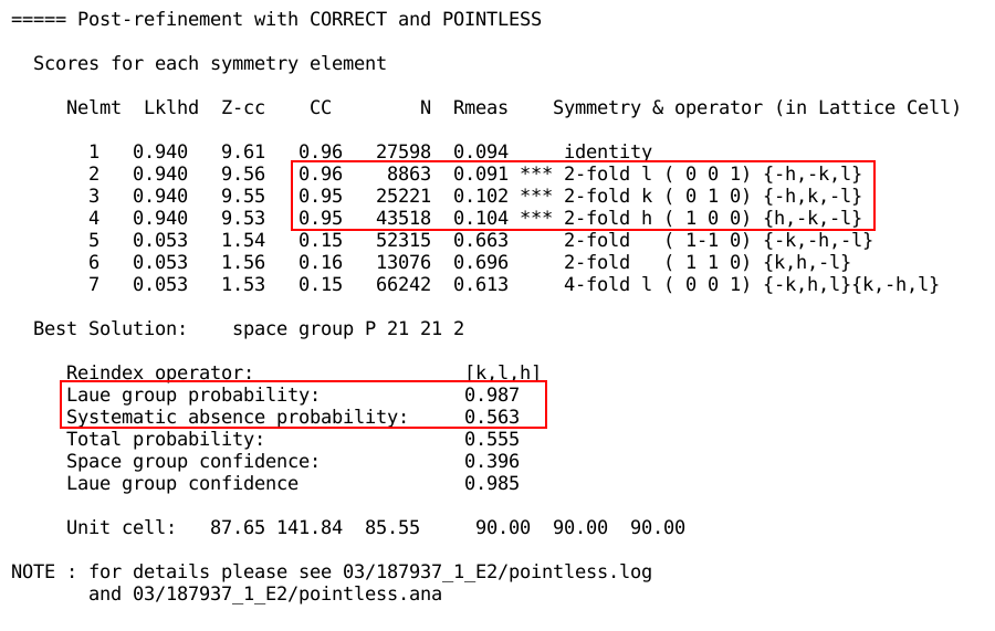
Space group assignment
Unless the space group for the crystal is already known (but even
then: surprises happen), the space group determination with POINTLESS should
be checked carefully. Ideally, all symmetry elements should have a
similar good score:
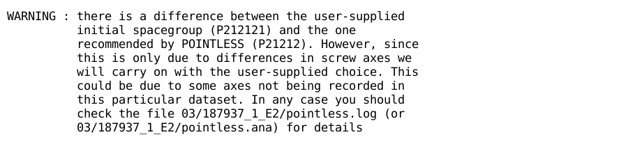
The reflections allowing for an unambiguous determination of screw
axes might not always be measured; this depends on the crystal
morphology, the way they are mounted and what possibilities for
re-orientation of the crystal are provided by the
beamline/instrument. If the space group was given on the command line
via the symm
parameter, or if a reference MTZ file was given with the -ref flag, the
user-provided space group will be compared to the POINTLESS analysis:
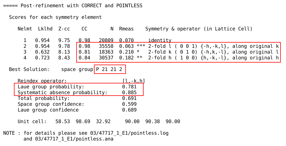
Sometimes, the space group assignment is unclear, a typical situation
being pseudo-orthorhombic unit cell dimensions and
non-crystallographic symmetries:
Here one 2-fold axis is significantly better than the other two,
showing the true space group as being rather monoclinic than
orthorhombic. If the user provided the space group (explicitly or
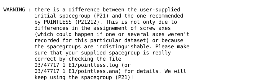
through a reference MTZ file), autoPROC will report any mismatch:
In this case the only way to find the "correct" space group
and cell is by solving the structure and reaching a full model with
good geometry and low R-values.
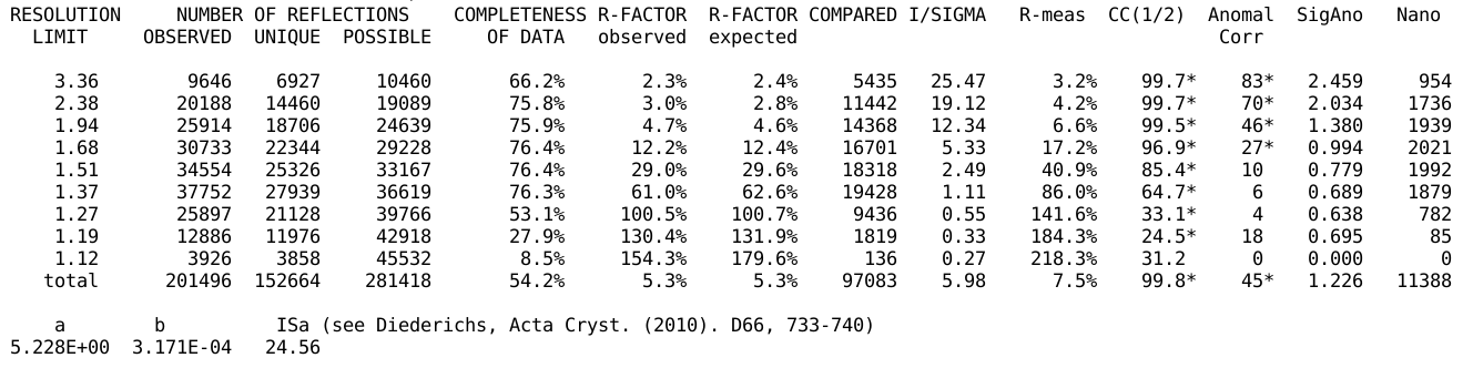
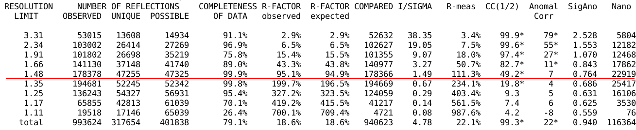
Statistics
At the end of the initial integration and space group
analysis/assignment, some statistics (as function of resolution) are
given:
It might already be obvious, that the crystal didn't diffract to the
corner (highest resolution) or even edge (where completeness is still
maximum) of the detector:
This is also visible in the diffraction picture itself:

top left (corner)
|
top left (edge)
|

top right (edge)
|
top right (corner)
|
In such a case using an explicit, initial high-resolution limit on the
command line
process -R 100.0 1.35 ...
would speed up data processing and ensure that not too many noisy
reflection data enter the final scaling/merging stage (which can
sometimes get stuck in a local minimum if the input data is too
noisy). But it is always best to choose a crystal-detector distance
that will use as much of the detector surface as possible for all
sweeps and orientations to be collected.
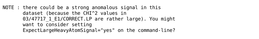
Anomalous signal
Furthermore, very strong anomalous signal is detected:
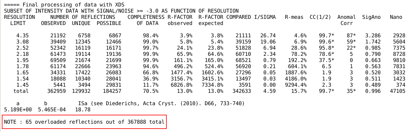
Overloaded reflections
Now that an initial set of parameters, a unit cell and space group is
available, a further round of integration and post-refinements is
done. This will give a similar table of statistics against resolution,
but also analyse for overloaded reflections:
Of course there should be as few as possible overloaded reflections:
these usually occur for the strongest, low-resolution reflections
which are the most important when it comes to structure solution via
molecular replacement, heavy-atom substructure solution for
experimental phasing, density-modification to improve phases and bulk
solvent modelling in refinement.
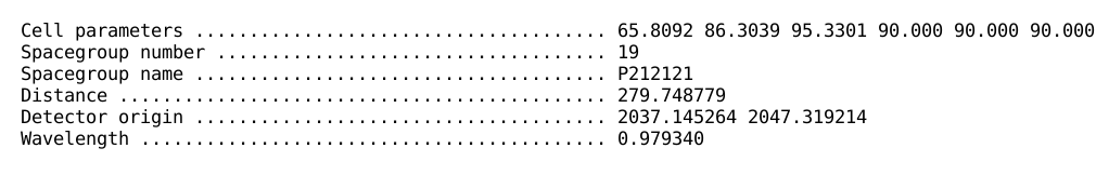
A short summary about cell parameters, distance, detector origin and
wavelength is also given:
Introduction to plots
There are several plots created that can be very useful in
interpreting data integration but also analyse the instrumentation
side of the experiment. Most of those are given as a function of image
number - but be careful: a consecutive image numbering might not
correspond to a consecutive collection of those images. If some kind
of interleaving was done (inverse-beam or interleaved wavelength)
there was additional exposure and data collection at specific wedge
sizes. Also, if the crystal was translated during collection - either
smoothly in a helical scan or step-wise to new positions on the
crystal - this needs to be taken into account when interpreting those
plots. here we will give some typical examples, but different
experimental designs might result in different plots.
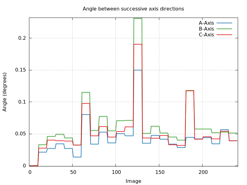
Changes to orientation matrix (angle_cell_axis_ABC.png and angle_cell_axis0_ABC.png)
The first set of plots is based on the orientation matrices determined
by XDS for each block
of images:
- angle_cell_axis_ABC.png: this shows the rotation
angle between orientation matrices of successive blocks of
images. We don't expect a large jump of this angle at any point,
since this would point to a sudden change of orientation during
rotation of the crystal.
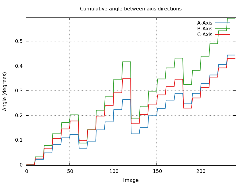
- angle_cell_axis0_ABC.png: similar to the above,
but now always using the orientation matrix of the first block of
images as a reference. We expect a smoothly varying, small set of
values over the full image range. An oscillating, but periodic (for
180 and 360 degree of rotation) behaviour might point to a
"wobbly" rotation axis.
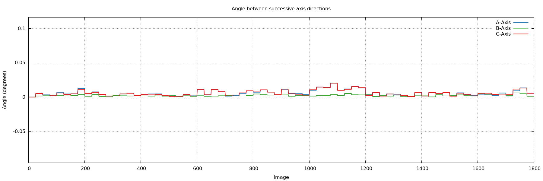
angle_cell_axis_ABC.png
ideal: very small change in orientation between blocks of images
|
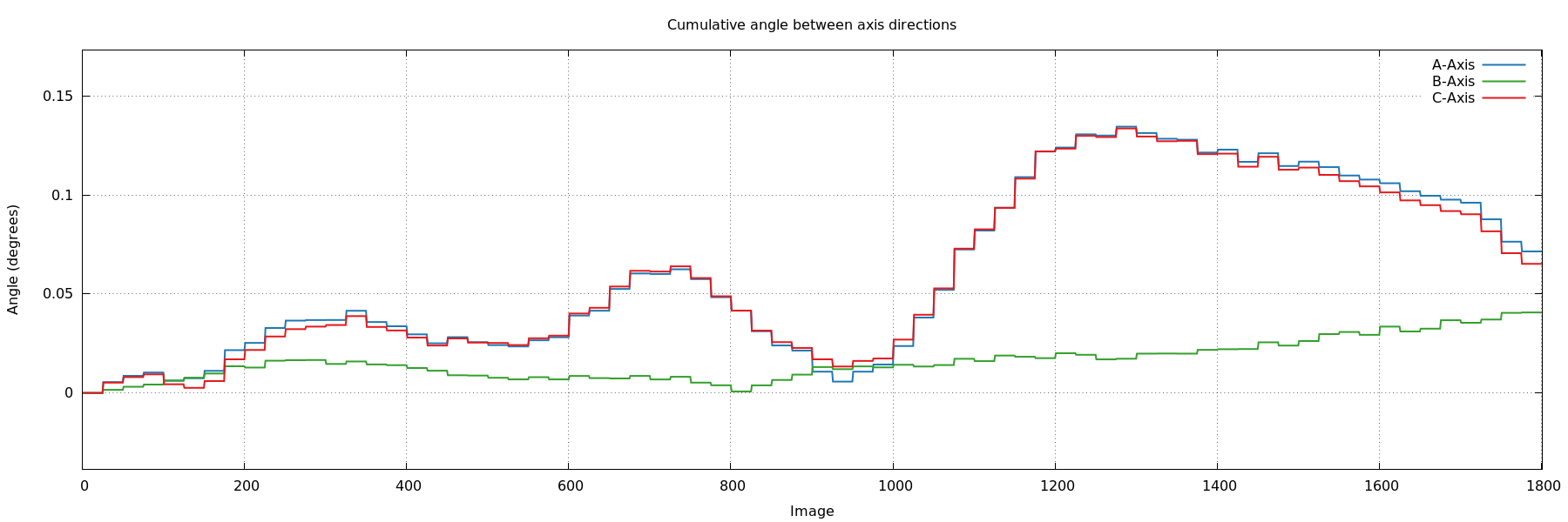
angle_cell_axis0_ABC.png
ideal: small and smoothly changing relative to first block of images
|
| |
| |
angle_cell_axis_ABC.png
interleaved energies (60 image wedge-size): problems getting back to
previous position after each wedge?
|
angle_cell_axis0_ABC.png
interleaved energies (60 image wedge-size): also an underlying trend
(relative to first orientation) - maybe different amount of increase
in cell axes due to radiation damage?
|
Change in cell dimensions/volume (cell_axes_devmean.png)
Another useful plot is the change of cell dimensions (axes) from their
respective mean as a function of image number. We expect a smooth,
hardly varying set of values. If radiation damage occurred and this
manifests itself as an increase in cell dimensions (see Ravelli et al,
2002), a steady increase in those changes could be observed:
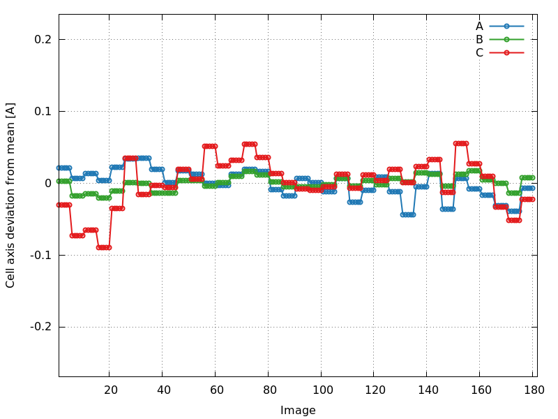
cell_axes_devmean.png
P2: good - hardly any change in cell axes
|
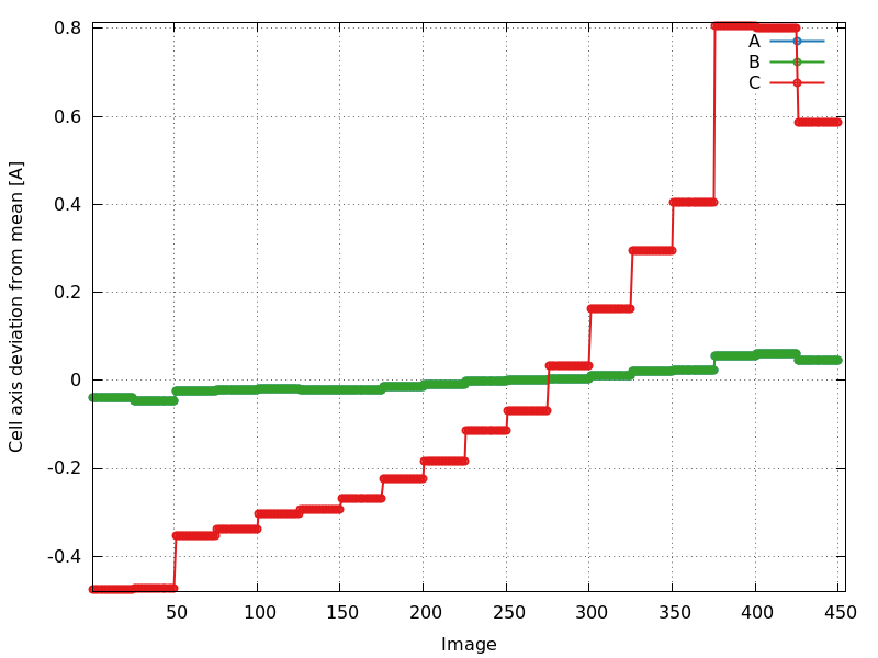
cell_axes_devmean.png
P6122: increase especially in c-axis
|
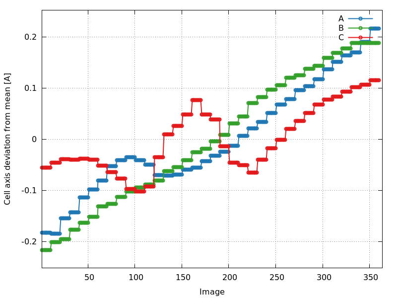
cell_axes_devmean.png
C2221: increase in all axes
|
Crystal to detector distance (distance.png)
The above plots do rely on an accurate determination of the cell
dimensions - which are highly correlated to the crystal-detector
distance. Any instability or drift in the distance parameter will
result in a drift of cell dimensions and could therefore lead to a
misinterpretation. autoPROC analyses the
distance refinement very carefully and will automatically switch off
refinement of this parameter if it shows instability during parameter
refinement:
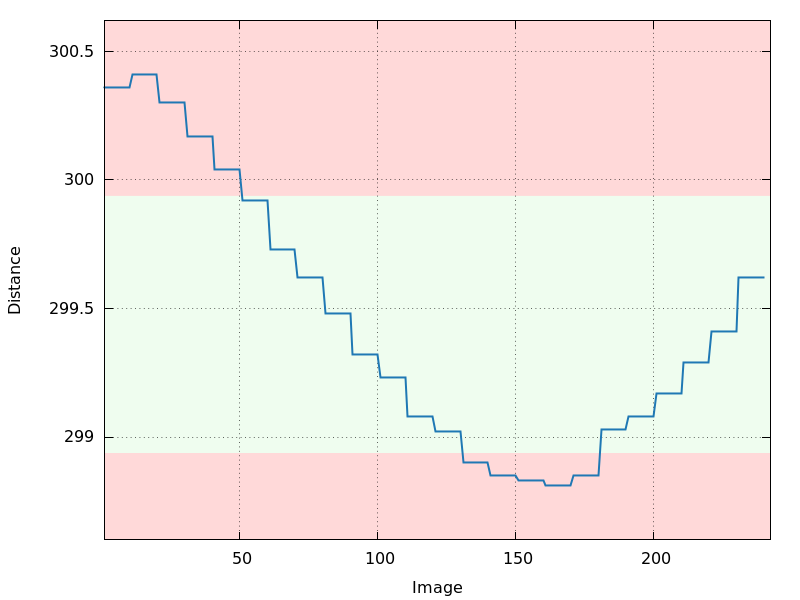
distance.png
120 degree of data: crystal centering slightly off?
|
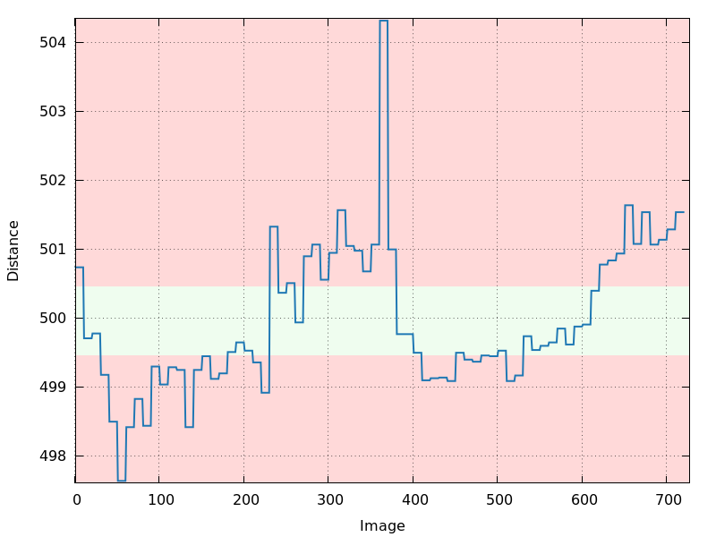
distance.png
180 degree of inverse-beam data: instability of parameter refinement
|
If the refinement of cell parameters was disabled during the
integration step (as is the XDS default since BUILT=20170720),
a steady decrease of the distance parameter can be due to a steady
increase in the unit cell dimensions due to radiation damage. The
distance refinement tries to compensate for this and acts as a
"proxy" to the detection of radiation damage.
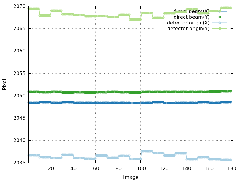
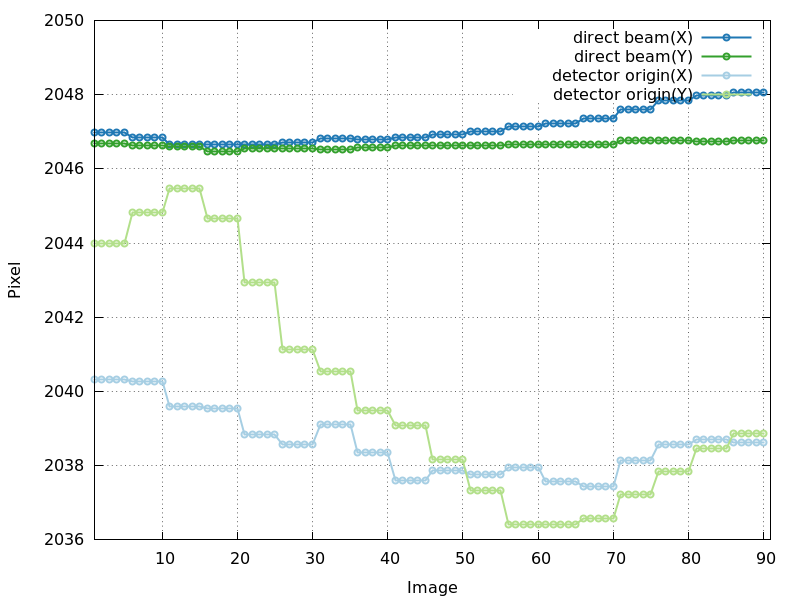
Direct beam position and detector origin (detector_center_origin.png)
The direct beam position and the detector
origin (both expressed as a position on the image) are usually
quite stable during refinement. But one can still extract information
from those plots:
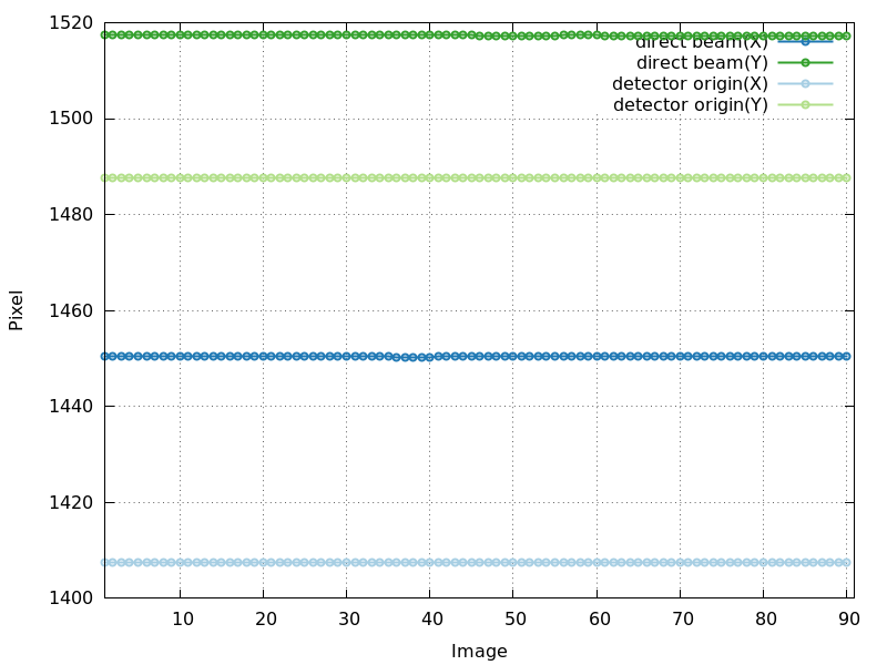
detector_center_origin.png
good - very stable over whole image range
|
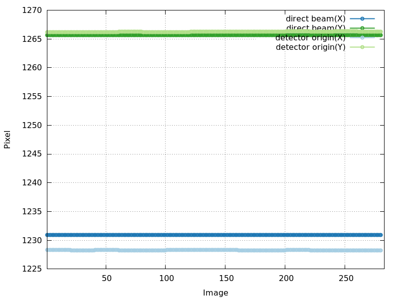
detector_center_origin.png
good - very stable (but values for detector origin and direct beam
quite apart: incident beam and detector plane normal not parallel
(due to detector alignment)
|
detector_center_origin.png
good - very stable (and values for detector origin and direct beam
very close: very accurate alignment of detector plane to incident
beam)
|
| |
| |
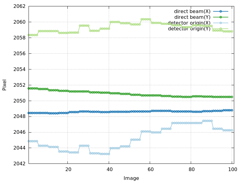
detector_center_origin.png
drift in direct beam position - is this "real" (due to
real drift of beam at beamline)?
|
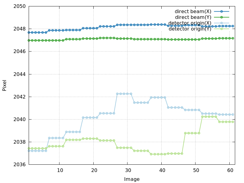
detector_center_origin.png
direct beam position quite stable, but detector origin refinement
unstable
|
detector_center_origin.png
drift in direct beam position and very unstable detector origin refinement
|
Standard deviation on spot position and spindle value (standard_deviation.png)
All of the above parameter refinements will add up to values of
standard deviation for spot position and spindle value. This can be
taken as a kind of "summary" to point to problematic image
ranges or patterns. But the exact interpretation of the underlying
reasons still requires careful inspection of the different plots
described above ... and ultimately the diffraction images themselves
including the predicted spots and spot shapes.
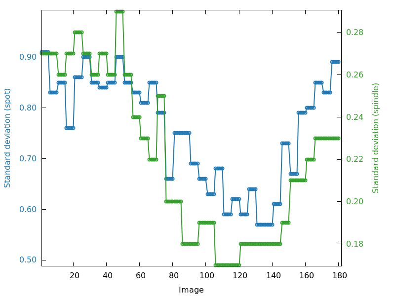
standard_deviation.png
poorer region at beginning (around image 30) than around image 120
|
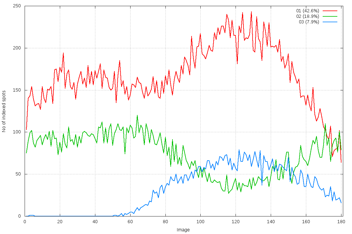
run_idxref_spot_hkl_hist.png
multiple lattices: 3 distinct indexing solutions visible around image 120
|
GPX2
central region of image 30
|
GPX2
central region of image 120
|
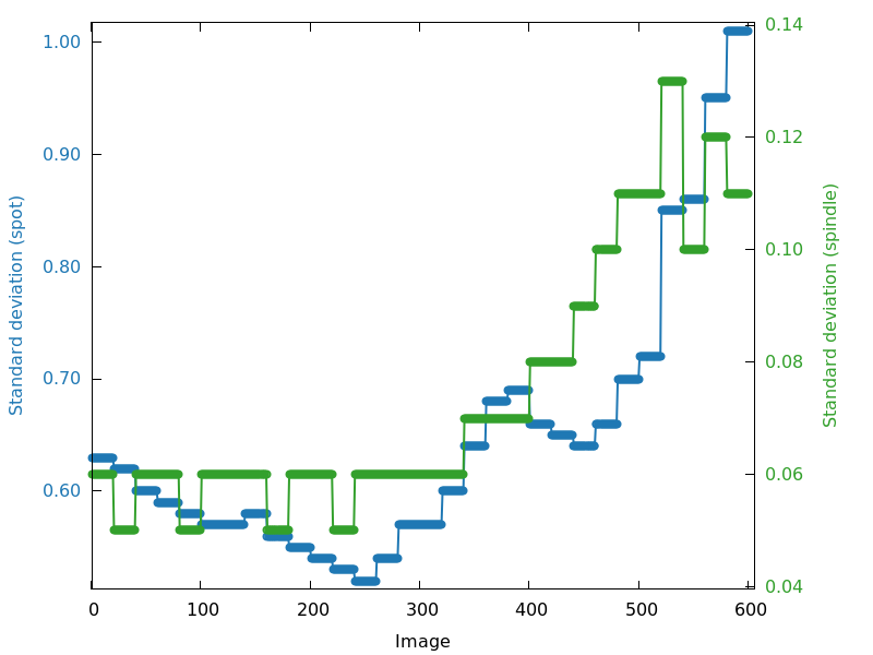
standard_deviation.png
poor towards the end
|
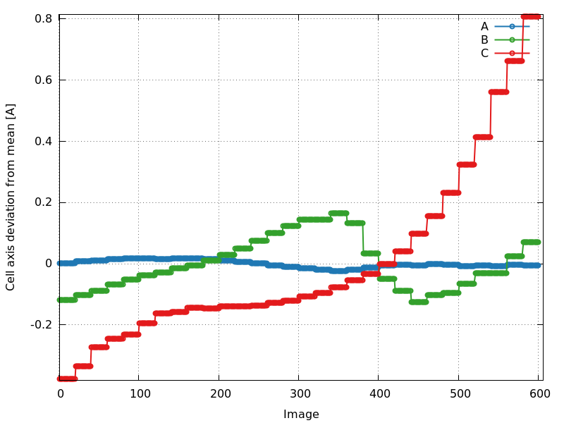
cell_axes_devmean.png
increase in cell volume
|
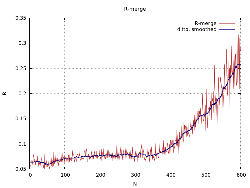
ana_aimless_Rmerge.png
increase in Rmerge
|
At this point, autoPROC will usually scale each sweep of data
internally, merge symmetry-related reflections and create merged
reflection files in MTZ and Scalepack format (see also parameter autoPROC_ScaleEachDatasetSeparately). For
multi-sweep datasets those results might not be used in the end, but
if not all sweeps are of equal quality (especially in the case of
radiation damage) this might allow checking and working with each
separate sweep.
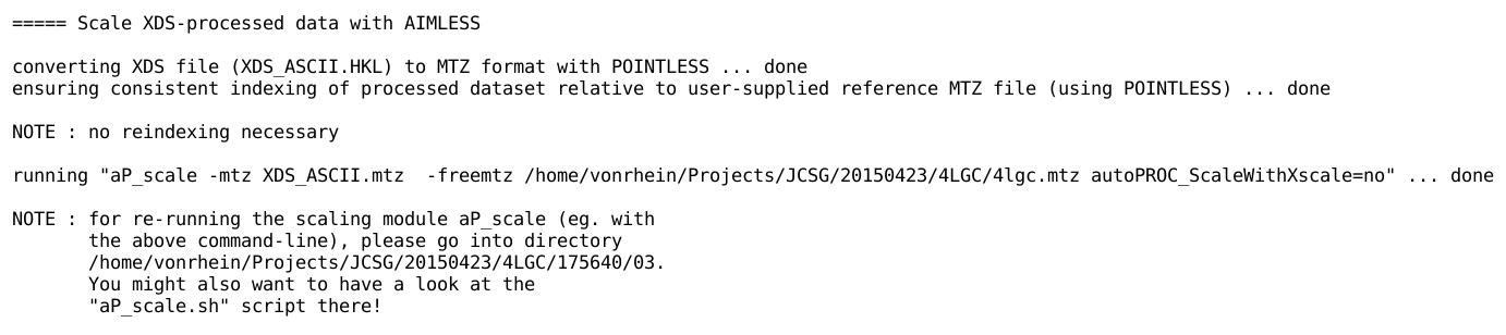
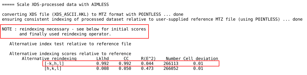
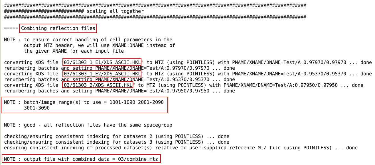
First autoPROC reports about file conversion, (potential) re-indexing
requirements and gives a pointer to the actual command run for the
scaling module:
If a reference reflection MTZ file was given, POINTLESS is used
to check for possible re-indexing
requirements. This will ensure that the output reflection data
from autoPROC is consistent with the reference given by the user -
which will simplify usage of autoPROC results in pipelines like Pipedream.
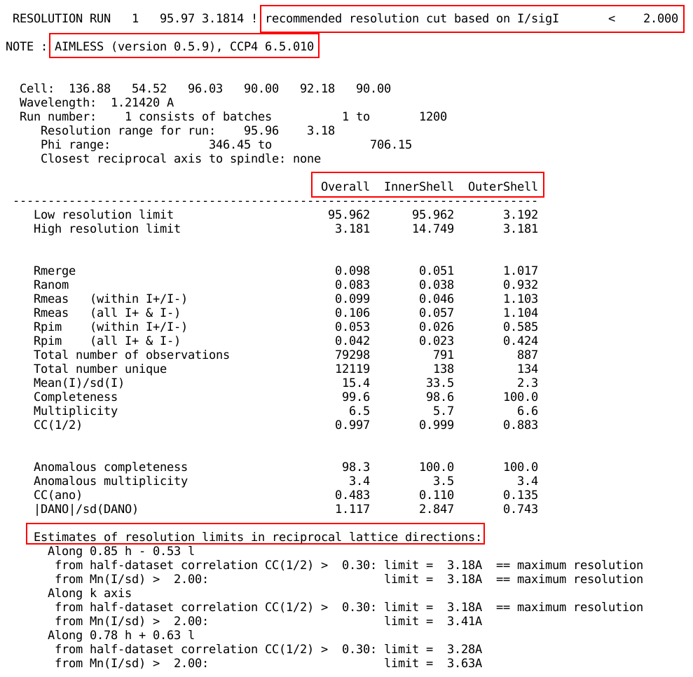
Overall statistics for AIMLESS scaling
If scaling was done with AIMLESS, the
program version used, a table containing various statistics for
overall, inner and outer resolution shell and some analysis about
anisotropy of diffraction are given:
These are for all reflections used in the scaling procedure, i.e. up
to the isotropic high-resolution limit determined using the criteria
described below. It therefore corresponds to the
"traditional" way of looking at data: using isotropic
resolution bins to compute statistics for all measured reflections
within each resolution bin. Of course, in case of general anisotropic
diffraction this is a limited view and describes data rather poorly -
which is where STARANISO comes into
play with its general analysis of anisotropy.
High-resolution criteria
autoPROC will automatically decide on an appropriate high-resolution
limit based on various criteria (I/sigI, CC(1/2), Rpim, Rmerge,
Completeness). Because any change of the high-resolution limit might
result in a different behaviour of the internal scaling step (a
different set of reflections is used by the refinement procedure), an
iterative procedure is applied:
- for each criterion (e.g. I/sigI or CC(1/2) value) a series of value pairs is given
- the first value applies per "run"
- the second value applies to the data resulting from an (optional) collection of "runs"
- this dinstinction comes into play for multi-sweep datasets where several sweeps might get merged into a single dataset (see below)
- each cycle of the iterative scaling procedure will use the corresponding criterion from this list (or the last one if more cycles are run than values given)
- the actual values in this list usually move from a looser to an ever tighter value until the last item in the list corresponds to the final value autoPROC should aim for
- autoPROC will often not get the intended criterion value absolutely spot-on: because of interpolation and binning it is possible that e.g. the final I/sigI value in the highest shell will actually be 2.1 instead of the intended 2.0.
The current default values for the various criteria are
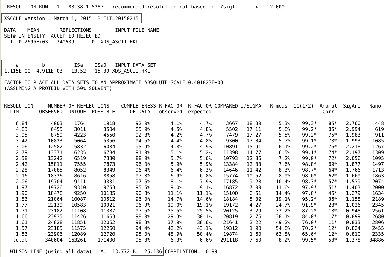
Overall statistics for XSCALE scaling
If scaling was done with XSCALE
(see autoPROC_ScaleWithXscale),
the program version used, a detailed table of statistics (as function
of resolution), the I/sigI(asymptotic)
(ISa/ISa0) and the Wilson B-factor are given:
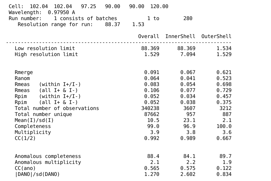
Then the same table containing various statistics for
overall, inner and outer resolution shell is shown - to give an easy
comparison between different scaling approaches:
This is again using the "traditional" approach of isotropic
resolution bins, i.e. looking at all reflections used in scaling up to
the high-resolution limit defined by the above
criteria.
STARANISO
Once the data has been scaled (either via AIMLESS or XSCALE) using a
"traditional" isotropic viewpoint, those scales are then
applied to all input data in order to have a scaled but unlimited set
of reflection data for the analysis of anisotropy via STARANISO.
Due to the scaling program specifics, there is a small difference at
that stage:
- the AIMLESS scaling will apply the various high-resolution criteria iteratively until
convergence and the resulting (final) scale and error-model
parameters are applied to the full input data;
- since XSCALE doesn't provide this functionality, the first
scaling result (on the original, full input data) is used for the
following step
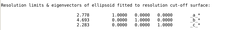
The resolution limits along the principle axes of the fitted ellipsoid
are a good way of describing the approximate limits of diffraction
(and resolution). Please be aware that the exact shape of the
observation surface does in general not need to follow an ellipsoid:
see the STARANISO
manual for all details.
Overall statistics for measurements
Once STARANISO has analysed the full,
scaled reflection data, it will arrive at a high-resolution limit to
which there is significant signal in the data. This is based on a
local <I/sd(I)> analysis and a fitted ellipsoid. All
measurements up to that high-resolution limit are then used to compute
merging statistics.
Please note that these merging statistics do not correspond to any
output reflection file and are presented here only to help
understanding the move away from the "traditional" isotropic
analysis (see above) to the anisotropic analysis as done by STARANISO. In case of significant
anisotropy it can show that using an isotropic resolution cut results
in the inclusion of noisy reflections - and in poor merging statistics
at high resolution. On the other hand, using the results of a full
anisotropic analysis of significant data (i.e. observations) it becomes obvious that
these provide real signal and excluding those in the
"traditional" isotropic approach (either via AIMLESS or XSCALE scaling) means excluding real
information.
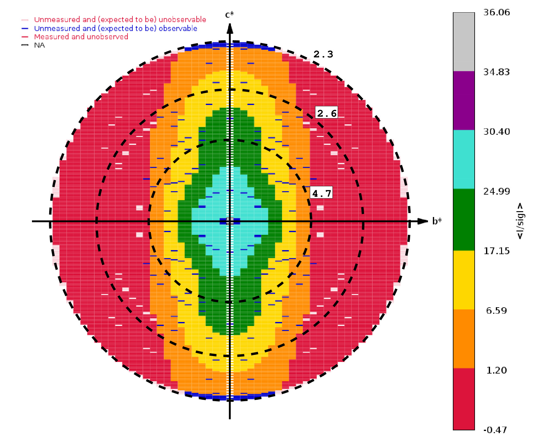
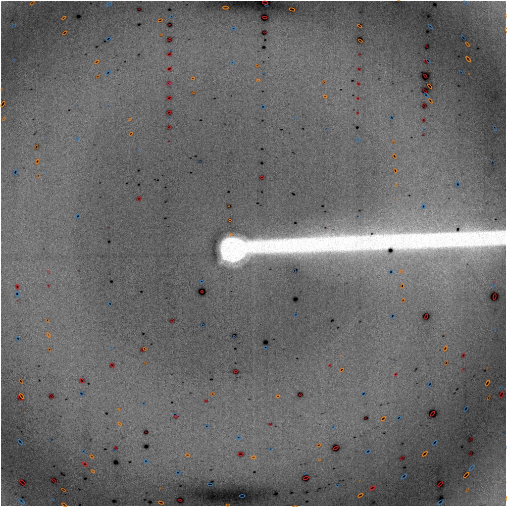
In one example (5SZQ)
the isotropic analysis decided on a high-resolution limit of 2.6 Å -
while the STARANISO analysis shows the degree of anisotropy (2.3 Å in
the best direction and 4.7 Å in the worst):
The different classes of reflections in the above picture are given
different colors to help visualising the anisotropy of the
data. Different views in reciprocal planes and along principle axes of
the ellipsoid are given. The most important regions are:
- RED: these are unobserved (but measured) reflections
- ORANGE: measured and observed (i.e. still significant)
reflections
- BLUE: unmeasured but expected to be observable
reflections (i.e. missed significant data due to detector limits,
crystal-detector distance, gaps, cusp, ice-rings etc)
Overall statistics for observations
The merging statistics for all observations (i.e. measurements with a
significant local <I/sd(I)> value as determined by STARANISO) represent the correct way of
describing anisotropic data. This corresponds to the output reflection
files with a name of "*staraniso*".
REMARK 200 (remark200.pdb)
This table is also the basis for writing a REMARK
200 section into file remark200.pdb:
Introduction
autoPROC tries to handle multi-sweep datasets
fully automatical. For this some assumptions are made:
- All datasets given to a single autoPROC
("process") run come from the same crystal
mounted identically on the same instrument:
- any difference in settings (wavelength, distance, 2-theta,
goniostat, rotation range per image etc) between datasets
is described in the image header
- you might want to check with imginfo if
this is correct
- The final merging will combine all datasets that have the same
wavelength/energy value:
- since there could be small difference in the
wavelength/energy value written in the image header, the
parameter WavelengthSignificantDigits
allows the user to accommodate for this.
- to avoid confusion, you could use one of the
energy-wavelength conversion jiffies:
By default, the find_images utility is used for
finding sets of diffraction images and classifying them as distinct,
i.e. belonging to different sweeps. Since this is only based on file
names, it might not always give the desired result - in which case
using the -Id flag might
help. If a single sweep consists of image files following different
name templates, using symbolic
links to work around this might be necessary.
In any case, autoPROC will always report the distinct sweeps at the
beginning (and then goes on to process each sweep on its own):
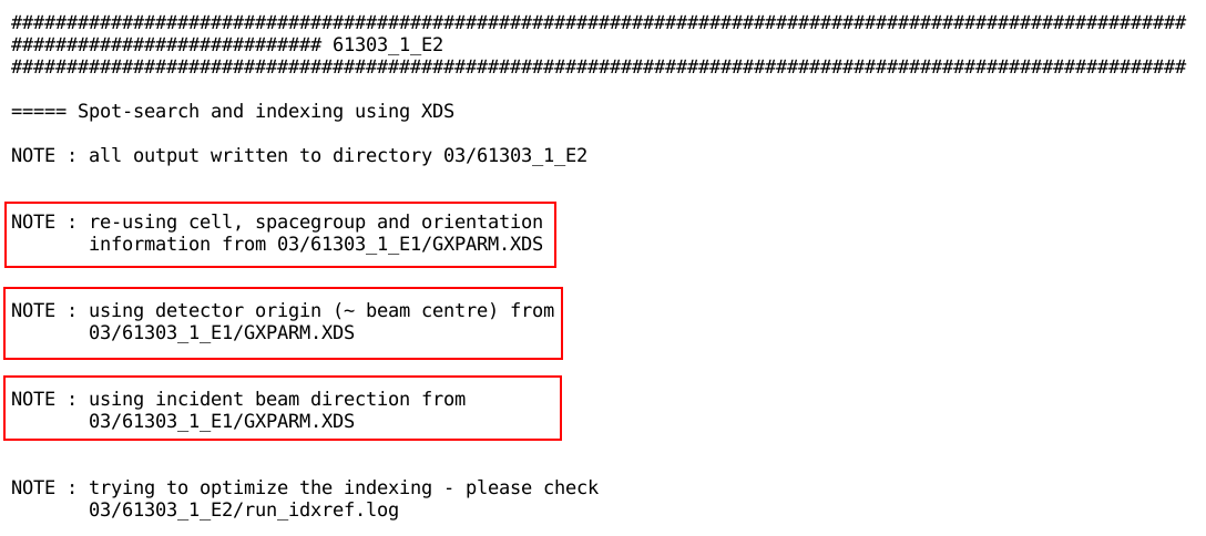
Effect on processing second and following sweeps
The effect of giving autoPROC several sweeps
of data becomes apparent for the second and all following sweeps:
autoPROC will
As one can see, the first sweep is taking on a special role - acting
as a reference for the others. The automatically determined order of
sweeps (by default based on timestamps in the image headers, which
would hopefully be accurate) might not be the best to use for this
approach. In this case, using the -Id flag would enable the
user to give a different ordering, with the "best" dataset
given first.
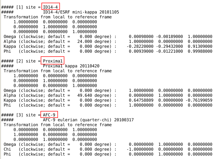
Multi-axis goniostats (kapparot)
One important requirement for the correct handling of multi-sweep
datasets with differing goniostat settings (that change the effective
orientation of the crystal) is an accurate description of the
goniostat axes. Only if these are known can autoPROC (via the kapparot program) transform the orientation matrix
of the reference sweep to the new goniostat settings - which is needed
since XDS
has no knowledge about multi-axis goniostats and treats the rotation
axis in a very generic way. We provide a pre-defined set of multi-axis
site definitions that can be listed via
x_kappa -list
some of which are shown here:
To use one of those site definitions, the parameter
KapparotSite needs to be set to the site identifier.
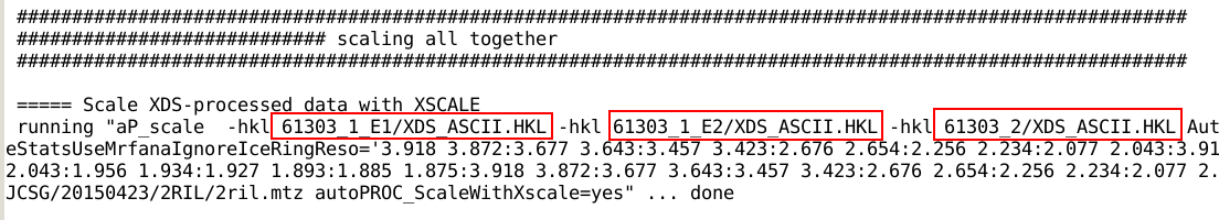
Final scaling and merging of all data
In the final scaling and merging step, the
integrated intensities of each sweep are used together. For the XSCALE
scaling path this is done by giving separate XDS_ASCII.HKL
files to the scaling module (aP_scale)
while for the AIMLESS path
autoPROC first needs to combine the individual reflection files using
combine_files:
To distinguish the data from different sweeps within that single
reflection file (a so-called multi-record MTZ
file), different BATCH
number ranges are used. Those then also need to be used when
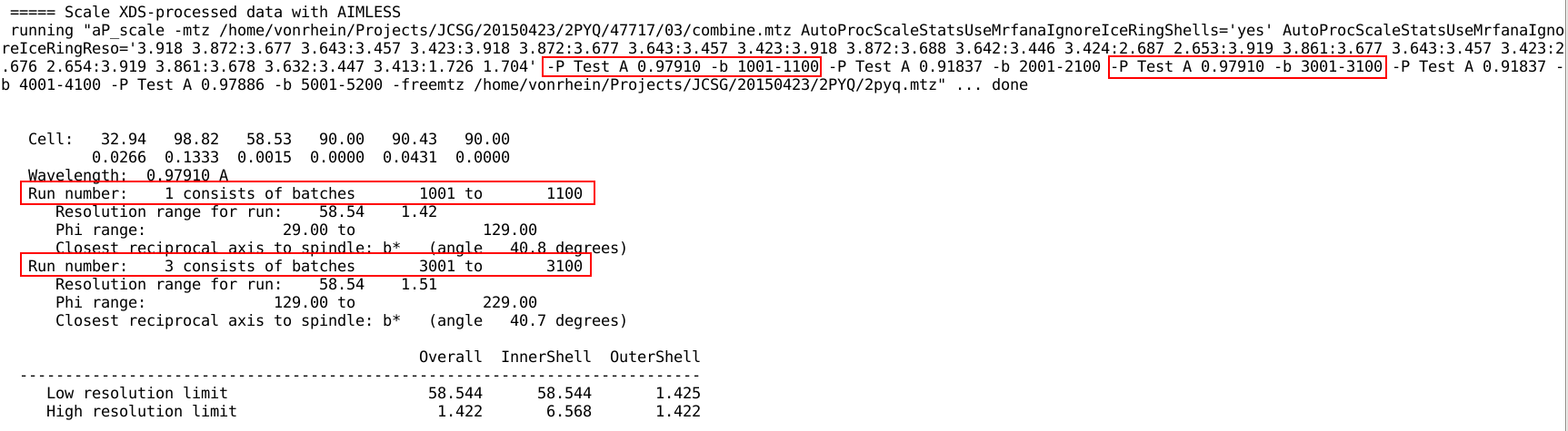
running the scaling module
(aP_scale) on that single reflection file:
At this point it is the dataset identifier given with
the -P flag to aP_scale that determines which sweeps are
being merged together at the end of the unified scaling
procedure. Remember that this defaults in autoPROC to the wavelength
value so that all sweeps collected at the same energy will finally be
merged together:
For the AIMLESS
path, some statistics are plotted as function of batch/image
number. In case of multiple sweeps collected at different energies,
separate plots for each wavelength are generated with the wavelength
(in Å) as part of the filename. E.g.
ana_aimless_0.91837_Bdecay.png        ana_aimless_0.97922_Bdecay.png        ana_aimless_0.97936_Bdecay.png
ana_aimless_0.91837_Bscale.png        ana_aimless_0.97922_Bscale.png        ana_aimless_0.97936_Bscale.png
ana_aimless_0.91837_Completeness.png  ana_aimless_0.97922_Completeness.png  ana_aimless_0.97936_Completeness.png
ana_aimless_0.91837_Rmerge.png        ana_aimless_0.97922_Rmerge.png        ana_aimless_0.97936_Rmerge.png
ana_aimless_0.91837_Scale.png         ana_aimless_0.97922_Scale.png         ana_aimless_0.97936_Scale.png
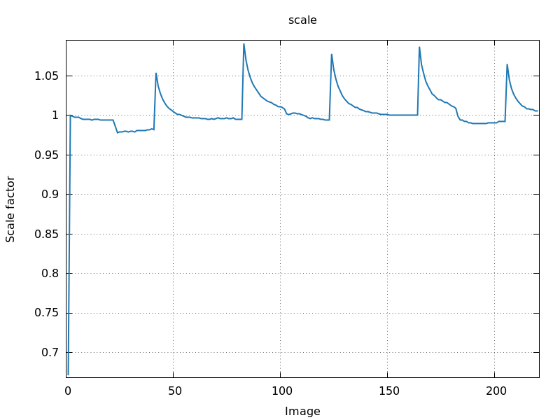
If multiple sweeps are merged together (because they were collected at
the same wavelength), this will be visible on those plots:
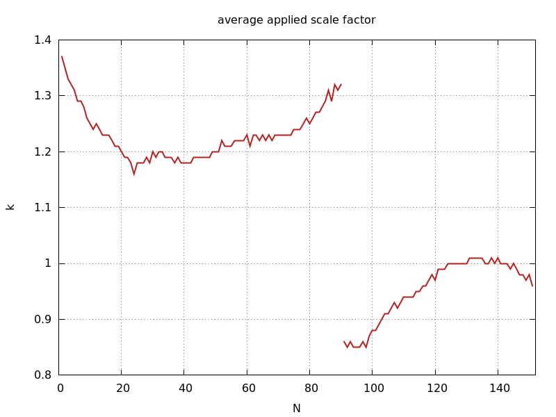
ana_aimless_0.97936_Scale.png
image scale factor
|
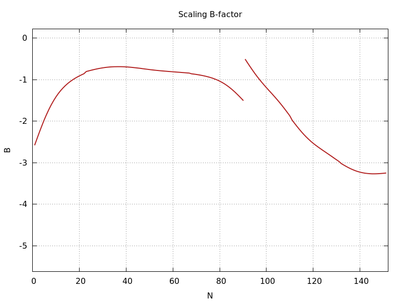
ana_aimless_0.97936_Bscale.png
scaling B-factor
|
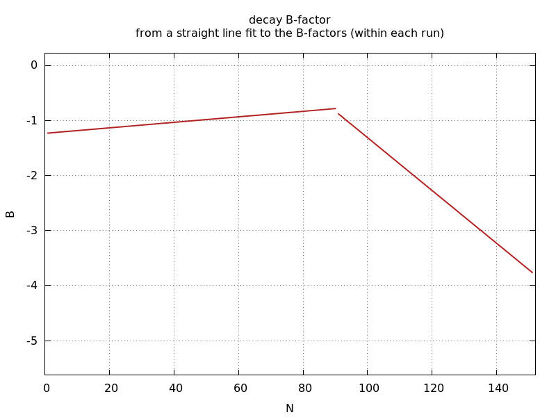
ana_aimless_0.97936_Bdecay.png
decaying B-factor (straight-line fit to scaling B-factor)
|
| |
| |
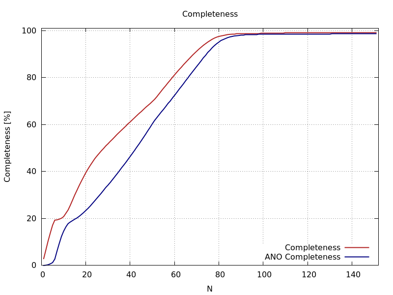
ana_aimless_0.97936_Completeness.png
cumulative completeness (overall and anomalous)
|
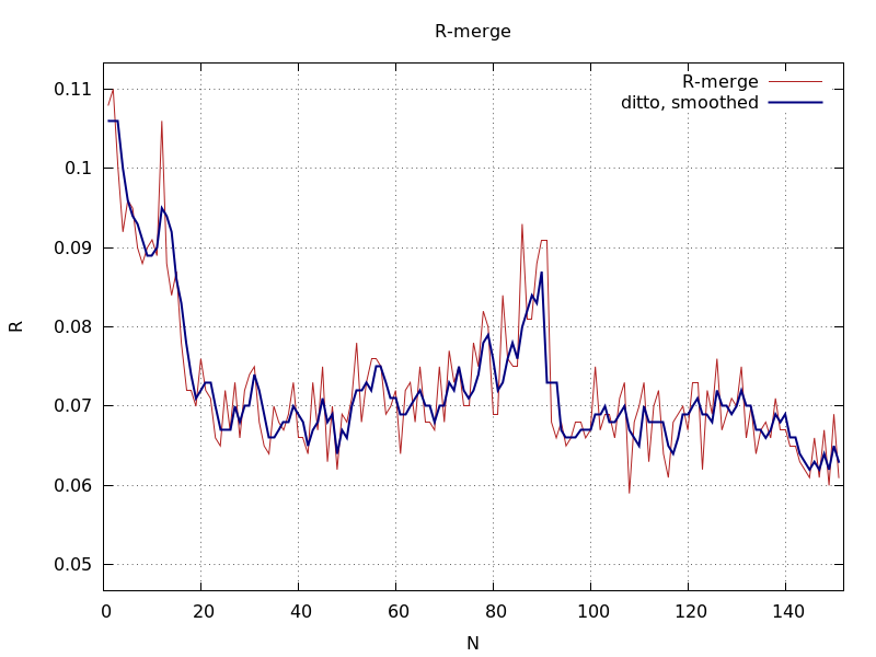
ana_aimless_0.97936_Rmerge.png
Rmerge
|
|
The final set of reflection data falls into two categories:
- "traditional" isotropic analysis
("truncate-unique.mtz")
- "new" anisotropic analysis with STARANISO
("staraniso_alldata-unique.mtz")
For multi-wavelength or (manually defined)
multi-sweep/crystal datasets, slight variations of those filenames can
occur - with the wavelength/dataset identifier inserted.
Each MTZ file should have a set of corresponding auxiliary files:
- "*.table1": merging statistics for innermost shell,
outer shell and overall
- "*.stats": merging statistics as a function of
resolution
- "*.xml": merging statistics in XML format
autoPROC generates a large number of plots using gnuplot. These are very useful in
analysing the final data quality, spotting problems or ways of
improving the data processing - even doing a better planing better for subsequent
experiments. Therefore it is highly recommended to ensure that a working
gnuplot installation is available on the machine running autoPROC.
The best way of looking at all these plots (including explanations and
notes) is the central "summary.html" file that is created in
the main output directory. It contains a structured index to easily
follow the flow of data through processing and highlights the final
files (that would go into subsequent steps of structure solution and
refinement) together with the relevant statistics (for deposition,
archiving and publication).
How to locate plots
One useful command to find the plots in the order they were generated
could be something like
process -I /where/ever/images ... -d 01 ...
ls -ltra `find 01 -name "*.png"`
which will list all PNG files in the order they were created.
How to view plots
There are a variety of tools available for viewing pictures in PNG or
JPG format. Some of the more popular options are the commands
display file.png
 - or -
qiv file.png
Obviously, you could also use your file manager to browse to the
relevant directory and file: after that a double-click (or whatever
the equivalent on your choice of operating system is) should open the
image for viewing.
Our visualiser for predictions
(position and shape) is called GPX2 and is invoked through
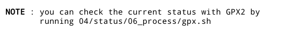
a series of scripts that will be generated automatically by autoPROC
throughout a data-processing. This will be reported on standard output
e.g. as
We use the notation of "status" to mean the visualisation of
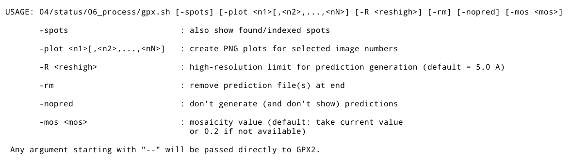
prediction positions and spot shape. This script can then be run -
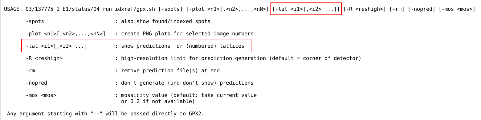
e.g. with the "-h" command-line argument to get a help
message (some values in that help message will be different depending
on the actual processing the predictions will be based upon):
Some command-line options are useful to discuss in more detail:
- -spots will not only show reflection predictions (as
computed from the current set of parameters and orientation),
but also the list of found spots;
- -mos <mos> allows the user to set a value
for mosaicity (which might be necessary at the indexing stage
since no value for mosaicity is available at that stage)
- -rm will remove the set of predictions after the user
closes the GPX2 window (this is required if a different
mosaicity value is to be used);
If the indexing step encountered the possibility of several lattices
or indexing solutions, several of these scripts will be generated: one
for each lattice/solution and one that allows visualising all found
lattices together.
 |
|
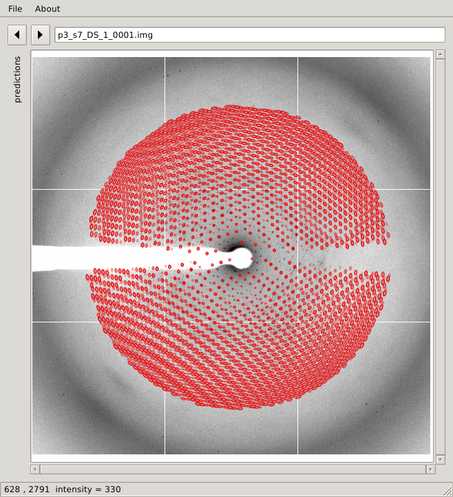
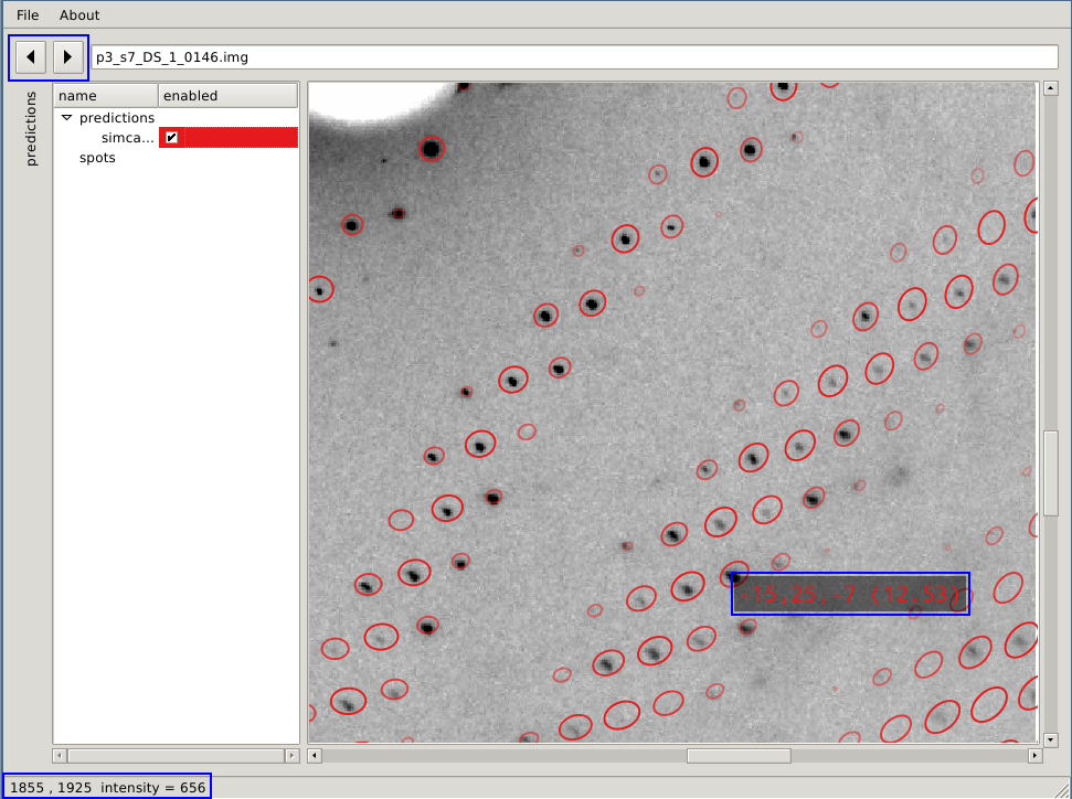
When running such a gpx.sh script, the GPX2 window will pop
up showing the full diffraction image and all prediction sets:
|
|
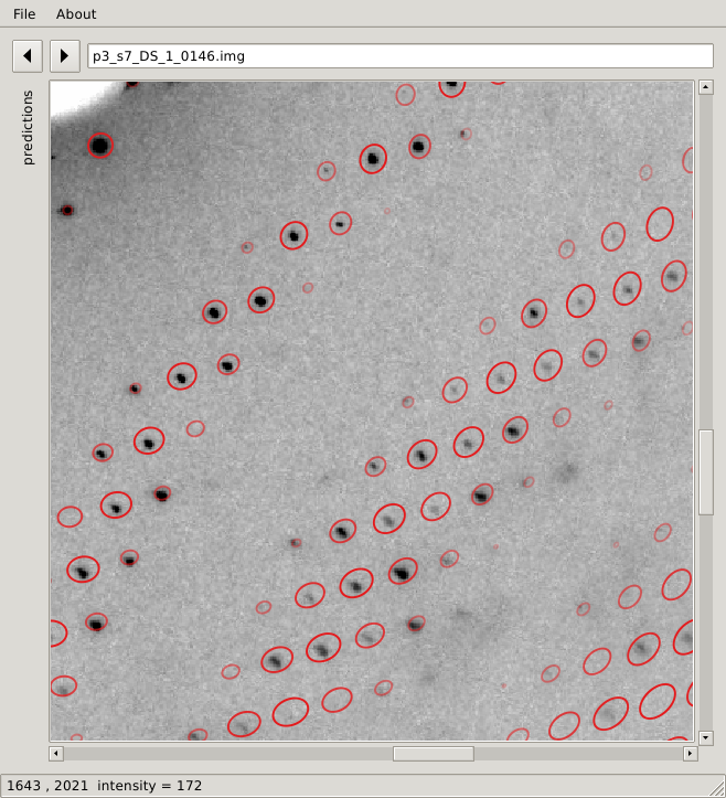
You can zoom in and out (centred under the current pointer position)
with the mouse-wheel and pan using the left mouse button:
|
|
| |
| |
|
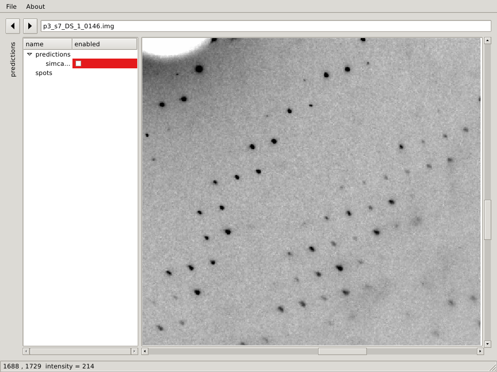
The prediction (and spot) sets can be switched on and off by expanding
the predictions text to the left:
|
- You can move between diffraction images using the arrow
buttons at the top left:
- the position and intensity value just under the pointer
position is displayed in the lower-left corner;
- Miller indices and resolution of a predicted reflection
are shown whenever the pointer moves inside one of the ellipses;
|
By default, a series of images will be generated at distinct angular
positions for each sweep:
Data processing, scaling and merging can produce a large number of
reflection files - which can be confusing to a user. Here we are going
to describe the different files produced by autoPROC (using the AIMLESS or XSCALE
scaling path).
| Scaling path |
File |
Description |
Remark |
Useful as input to the STARANISO server? |
| all |
INTEGRATE.HKL |
unmerged and unscaled intensities |
data for unpolarised beam (so a conversion to MTZ via POINTLESS needs to take this into account); error/variance model has not been adjusted |
possibly (since the unmerged protocol will convert this file to a multi-record MTZ file using POINTLESS before giving it to the "aP_scale" module from autoPROC) |
| all |
XDS_ASCII.HKL |
unmerged (and scaled) intensities |
polarisation correction has been applied and error/variance model is adjusted; scaling and outlier rejection has been applied (depending e.g. on the choice of correction factors) |
yes |
| AIMLESS |
XDS_ASCII.mtz |
unmerged (and scaled) intensities |
multi-record MTZ version of XDS_ASCII.HKL (via pointless -copy xdsin XDS_ASCII.HKL hklout XDS_ASCII.mtz) |
yes |
| AIMLESS |
aimless_alldata_unmerged.mtz |
unmerged and scaled intensities, no resolution cut |
scale factors, absorption correction and error model adjustments determined for the isotropically significant resolution range applied to all measurements |
yes (if the server is being told to not re-run the "aP_scale" step) |
| XSCALE |
xscale_alldata.ahkl |
unmerged and scaled intensities, no resolution cut |
result from first XSCALE step |
yes (if the server is being told to not re-run the "aP_scale" step) |
| XSCALE |
xscale_alldata_unmerged.mtz |
unmerged and scaled intensities, no resolution cut |
multi-record MTZ version of xscale_alldata.ahkl |
yes (if the server is being told to not re-run the "aP_scale" step) |
| AIMLESS |
aimless_alldata.mtz |
merged and scaled intensities, no resolution cut |
merged version of aimless_alldata_unmerged.mtz |
yes |
| AIMLESS |
aimless_alldata-unique.mtz |
merged and scaled intensities plus amplitudes: all measurements within sphere of highest observed resolution limit |
contains all measurements to the highest observed resolution limit as determined by STARANISO; amplitudes are derived by STARANISO via the French & Wilson method, using the correct anisotropic prior distribution of the expected intensity. |
no |
| XSCALE |
xscale_alldata.mtz |
merged and scaled intensities, no resolution cut |
merged version of xscale_alldata.ahkl |
yes |
| XSCALE |
xscale_alldata-unique.mtz |
merged and scaled intensities plus amplitudes: all measurements within sphere of highest observed resolution limit |
contains all measurements to the highest observed resolution limit as determined by STARANISO; amplitudes are derived by STARANISO via the French & Wilson method, using the correct anisotropic prior distribution of the expected intensity. |
no |
| AIMLESS |
aimless_unmerged.mtz |
unmerged and scaled intensities, isotropic resolution cut |
data up to the isotropic significant resolution range, i.e. this is the data the scale parameters used in AIMLESS are determined from |
no |
| AIMLESS |
aimless.mtz |
merged and scaled intensities, isotropic resolution cut |
merged version of aimless_unmerged.mtz |
no |
| all |
truncate.mtz |
merged and scaled intensities plus amplitudes, isotropic resolution cut |
result from running aimless.mtz through TRUNCATE |
no |
| all |
truncate-unique.mtz |
merged and scaled intensities plus amplitudes, isotropic resolution cut, complete data to highest resolution |
contains all reflections up to the highest resolution observation as well as a test-set flag |
no |
| all |
staraniso_alldata.mtz |
merged and scaled intensities plus amplitudes, anisotropic resolution cut |
result from running aimless_alldata.mtz through STARANISO |
no |
| all |
staraniso_alldata-unique.mtz |
merged and scaled intensities plus amplitudes, anisotropic resolution cut, complete data to highest resolution |
contains all reflections up to the highest resolution observation as well as a test-set flag |
no |
Last modification: 14.05.2018