MRFANA usage:

• Introduction

• Input files

• Binning

• Resolution & spacegroup

• Ice-ring handling

• Standard output
• Setup
• Statistics as a function of resolution
• Statistics as a function of image number

• Output files

• Some recommendations
• Equal-volume binning
• Equal-observation-number binning
• Traditional 1/d**2 binning
• Comparing different programs/pipelines

---

Introduction

MRFANA (which stands for Multi-Reflection File ANALYSIS) is our program for computing and analysing various data merging statistics as function of both resolution and image number (also known as "batch" number).

A basic help/usage message is displayed when running

mrfana -h
 

Here we describe the MRFANA version as distributed as part of autoPROC. This deviates in various aspects from the open-source version we released in October 2019: the latter is intended as a reference implementation of quality metrics computation.

---

Input files

MRFANA can read unmerged reflection data in various formats:

• from XDS:

• INTEGRATE.HKL:
• This file contains raw integrated intensities, i.e. unscaled and unmerged data.
• Be aware that the sigma values here have not yet been adjusted (this is done at the CORRECT stage).
• Therefore most statistics will be based on sigma estimates that are likely to be inaccurate .
• However, these might still be useful for the analysis of relative values throughout a dataset.

• XDS_ASCII.HKL:
• This file will contain scaled and unmerged intensities including CORRECT-adjusted sigma values.
• So-called misfits and aliens are marked by a negative sigma value - and are ignored upon input to MRFANA.

• XSCALE output files
• To write out (scaled) unmerged reflection files the MERGE= parameter needs to be set to "FALSE".

• MTZ files:

• Several programs like AIMLESS, POINTLESS or MOSFLM will write out unmerged MTZ files (or "Multi-Record MTZ" Files ... which is where MRFANA originally got its name from).

---

Binning

MRFANA can either be given an explicit list of resolution ranges for binning, or can determine these automatically.

For automatic determination, two command-line arguments can be used:

Flag	Argument	Comment
-n	number of bins (for equal volume binning)	a negative value will do the 'standard' binning on 1/d**2
-nref	number of measured reflections per bin (default=1000)	a negative value will trigger binning by equal numbers

If explicit resolution shells should be used, a comma-separated list of delimiting resolution values (in Angstroem) should be given to the -bins flag. E.g. using

mrfana -bins 10,5,3,2.5,2 ...

will create bins

  RL - 10.0 A
10.0 -  5.0 A
 5.0 -  3.0 A
 3.0 -  2.5 A
 2.5 -  2.0 A
 2.0 -   RH A

(where RL and RH are the low- and high-resolution limits of the input data, respectively).

Within autoPROC the default is to use equal-observation-number binning, i.e. running MRFANA with -nref -1000 (or similar).

---

Resolution & space group

MRFANA will compute the resolution of each reflection (H,K,L) using the unit-cell parameters stored in the reflection data. It will also use the space group given in the input file.

When using multi-sweep dataset files (e.g. from multi-wavelength or multi-orientation experiments) it is important to remember that the relevant sweep/dataset cell for each reflection will be used. This is done so that a resolution value reported in MRFANA can be used as-is when e.g. going back to individual sweeps/datasets (that each carry their own set of unit-cell parameters).

---

Ice-ring handling

Within the decision making process of an autoPROC run, MRFANA will by default treat ice-ring resolution shells differently. The default list of ice-ring resolutions is

3.906-3.873 A
3.671-3.642 A
3.450-3.420 A
2.681-2.649 A
2.258-2.235 A
2.076-2.056 A
1.955-1.936 A
1.922-1.906 A
1.888-1.872 A
1.721-1.713 A
1.524-1.519 A
1.473-1.470 A
1.444-1.440 A
1.372-1.368 A
1.367-1.363 A
1.299-1.296 A
1.275-1.274 A
1.261-1.259 A
1.224-1.222 A
1.171-1.168 A
1.124-1.122 A

and can be switched off via the -noice flag. This treatment has no effects on the computation of statistics and is only relevant within the context of the autoPROC scaling module.

---

Standard output

Standard output is organised in three main sections:

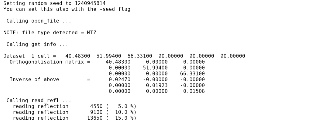
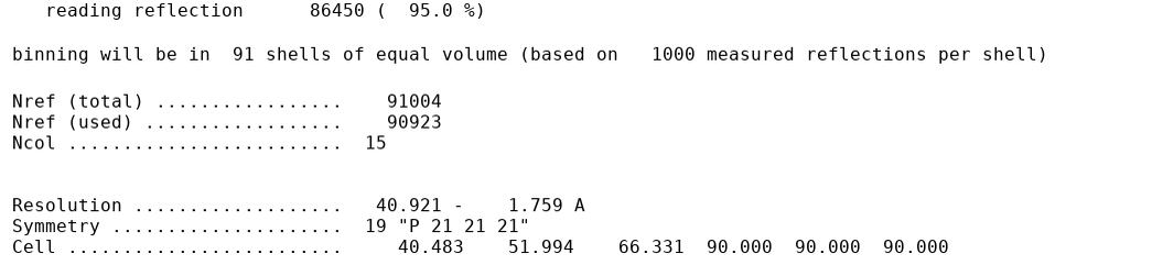
Setup

Here we report the information read from the reflection data, whether the data needs to be (re)sorted, details about space group and unit-cell dimensions and the random number seed used (relevant for the computation of the random half-set statistics CC1/2 and CCano).

Depending on the binning method used, the exact bin-defining resolution values are reported here as well.

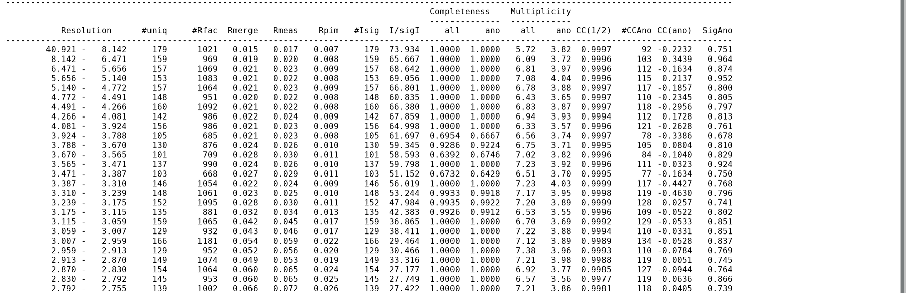
Statistics as a function of resolution

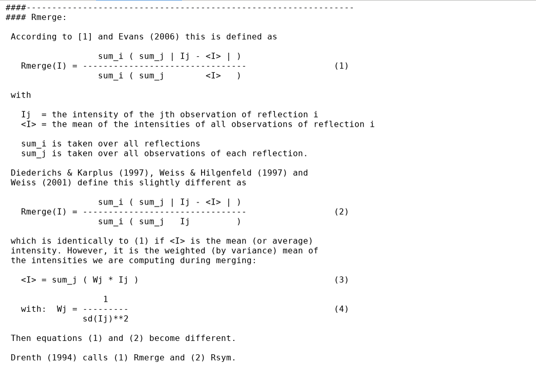
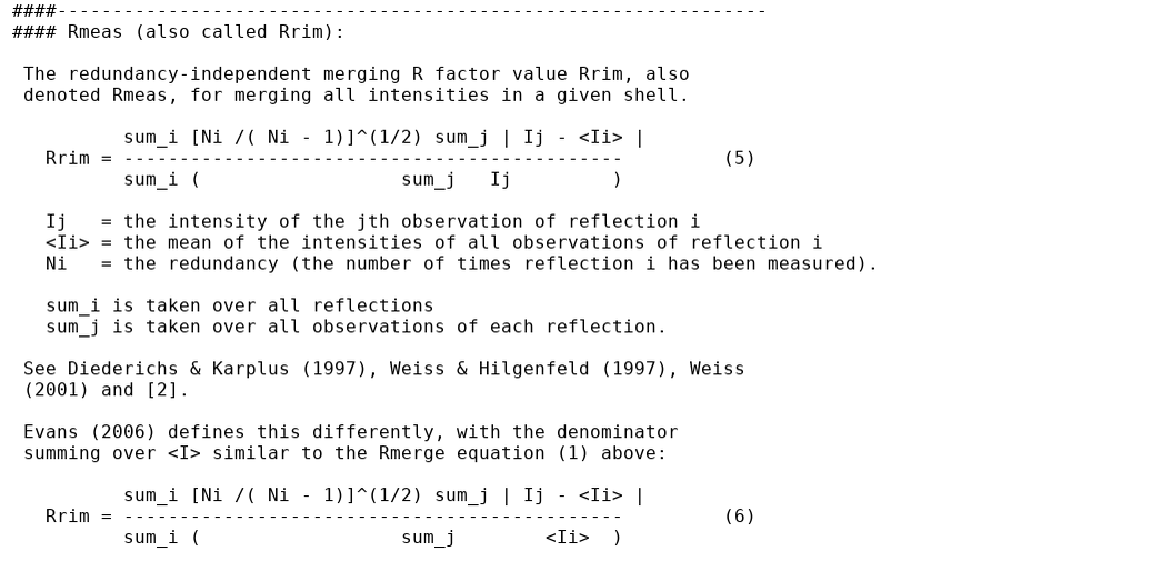
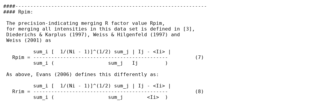
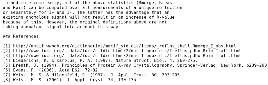
Some background information about R-values is given here:

This is given in two tables: (1) in full detail for all resolution shells

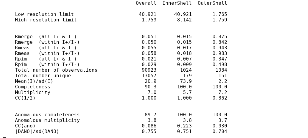
and (2) in a "Table 1" style summary for the inner, outer and overall shells.

For single-sweep datasets those two tables can be extracted e.g. with the following commands:

awk '/Completeness    Multiplicity/,/^ Total/' mrfana.log
awk '/Number of active ice-rings/,/DANO/' mrfana.log

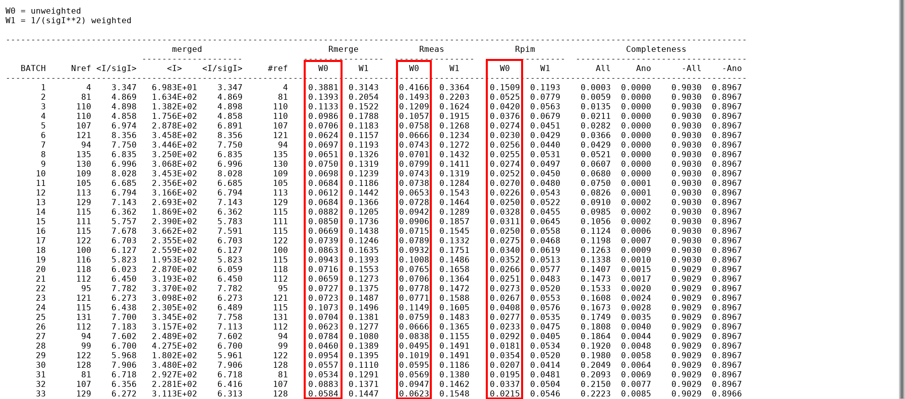
Statistics as a function of image number

This can be extracted via

awk '/merged [ ]*Rmerge/,/^   Total /' mrfana.log

e.g. for subsequent plotting of statistics (as a function of image number).

---

Output files

An ISPyB-compatible XML file can be requested using the -xml flag: here the (base) name of the output file should be given (for multi-sweep/multi-dataset/multi-wavelength data an appropriate naming convention will be used).

---

Some recommendations

The different binning methods all have their advantages and disadvantages, and which one should be used will depend on the question we are asking about a particular dataset (or a collection of datasets or processing results).

Equal-volume binning

Using the MRFANA default (positive integers given to -n or -nref) has the advantage of using the same number of possible unique reflections in each resolution bin. So if we are (1) interested in statistics - especially completeness - within isotropic resolution shells and (2) want to have the same number of possible unique reflections within each shell, then this could be the mode to use. It will ensure that the same number of (possible) reflections is available within each bin - so that various statistics can be computed with enough data points.

However, this will most likely result in rather wide bins at low resolution and maybe rather thin bins at high resolution (especially for very high resolution data) - which might be adequate for plotting reliably and consistently determined statistics as a function of resolution assuming that the crystal diffracted isotropically.

Equal-observation-number binning

This is very similar, in terms of the underlying idea, to the equal-volume binning described above, but without assuming that the crystal diffracted isotropically and/or that all possible data was collected with the same level of coverage across the full resolution range. Anisotropy, partial sweeps, missing data due to the cusp or shadowing can all introduce deviations from the ideal picture of complete isotropic data. This mode (via a negative integer given to the -nref argument) will ensure that the same number of actually observed (i.e. both measured and significant) unique reflections is used within each bin, leading to automatically self-adjusting resolution bin widths throughout the whole range.

When dealing with highly anisotropic data (e.g. analysed by STARANISO as part of autoPROC or from the STARANISO webserver) this would be our recommended mode - and what is used by default within autoPROC itself.

Traditional 1/d**2 binning

Both of the above binning methods have the disadvantage of (usually) giving rather wide bins at low resolution. If the emphasis is on analysis of the low resolution range of a dataset (e.g. to look for anomalous signal or because the crystal only diffracts to low resolution), then a smaller number of unique reflections at low resolution is probably better suited: this type of binning will provide for that. It can be triggered via a negative integer given to the -n argument.

However this binning mode will give rise to shells of increasing volume with increasing resolution, so that the number of unique reflections being used in those higher resolution shells can rapidly increase to very large numbers - which might not give enough detail at this opposite end of the resolution range.

Comparing different programs/pipelines

Comparing the results from different integration programs (like XDS, Dials, MOSFLM) or pipelines/tools (like autoPROC, Xia2, Grenades, fastDP, XDSGUI, XDSAPP and many more) can be very difficult because programs (1) use different methods at various stages, (2) have different default assumptions of the kind of experiment, detector, crystal and data quality they are encountering and (3) present the data quality descriptors in myriads of ways and formats, according to differing formulae. By using MRFANA on the scaled and unmerged results of each procedure, at least any variation in definitions and methods of computations for the relevant data quality metrics is taken out of this equation.

The "only" remaining issue is to ensure that identical binning is used across all reflection data files produced by the various programs/pipelines. One possible approach could be to

• run MRFANA with equal-observation-number binning on the sparsest dataset (the one with the lowest high-resolution limit and lowest completeness);
• this can be used as a reference for defining
• the highest common resolution limit (since all other datasets will be of at least that resolution or higher);
• the binning to be used;

• then run all other datasets through MRFANA using
• -r 999.9 highres (to only compute statistics to the common high-resolution limit);
• -bins ... to set explicit resolution bins (the relevant comma-delimited line can be extracted from the initial MRFANA run above;

This would ensure that all statistics can be compared between the different result files. Of course, results that suggest higher diffraction limits will not be taken into account within this comparison - and maybe some additional MRFANA jobs need to be run on a subset of the available results.

In general, one should be very careful not to over-interpret small differences in the data quality metrics obtained in this way: we are probably at least comparing apples with apples, but there are still distinct varieties available (e.g. small differences in unit-cell dimensions will result in reflections being assigned to different resolution bins for different result files).