TutorialMontevideo2013

UNDER CONSTRUCTION (throughout the workshop)

Content

• Introduction
• Local setup

• 1o22
• autoPROC (data processing)
• SHARP/autoSHARP (experimental phasing and structure solution)
• BUSTER (structure refinement)

• own data
• autoPROC (data processing)
• SHARP/autoSHARP (experimental phasing and structure solution)
• BUSTER (structure refinement)

---

Introduction

These pages are intended as a resource for the tutorials of our software at the International workshop, Joint CeBEM-CCP4 initiative, April 9th-17th, 2013, Institut Pasteur Montevideo, Uruguay .

Much more introductory material is available for each program:

• autoPROC (data processing)
• SHARP/autoSHARP (experimental phasing and structure solution)
• BUSTER (structure refinement)

autoPROC relies on external programs like:

• XDS: Kabsch, W. XDS. Acta Cryst. D66, 125-132 (2010).
• POINTLESS, SCALA/AIMLESS: Evans, P. (2006). Scaling and assessment of data quality. Acta Cryst. D62, 72-82.
• CCP4: Collaborative Computational Project, Number 4. 1994. "The CCP4 Suite: Programs for Protein Crystallography". Acta Cryst. D50, 760-763.

---

Local setup

All programs should be configured and setup correctly. You can test this by running

% process -h

For running this tutorial, it might be a good idea to start in a fresh, empty directory.

---

1o22

This should be a reasonably fast run through all stages of data-processing (about 5 min on an i7-2720QM laptop with 8Gb of memory).

We're going to use the data for 1O22 from the JCSG. It is

• a 170 residue protein
• expressed with Se-MET (6 Met in sequence)
• data collected at the peak wavelength (0.9778 A)
• a fluorescence scan gave values of f'=-7 and f"=5.0
• detailed information available here
• Images available online at Protein Diffraction

autoPROC (data processing)

Note: more examples and tutorials are given on the autoPROC wiki. And make sure you have a copy of the autoPROC reference card.

This peak dataset consists of 90 images (tm0875_8p44_1_E1_001.img to tm0875_8p44_1_E1_090.img). A quick look at the image header can be done with

% imginfo ~/Desktop/Tutorials/1o22/tm0875_8p44_1_E1_001.img

that gives

>>> Image format detected as ADSC

===== Header information:
date                                = 13 Oct 2002 18:47:43
exposure time             [seconds] = 45.000
distance                       [mm] = 200.000
wavelength                      [A] = 0.977800
Phi-angle (start, end)     [degree] = 90.000 91.000
Oscillation-angle in Phi   [degree] = 1.000
Omega-angle                [degree] = 0.000
2-Theta angle              [degree] = 0.000
Pixel size in X                [mm] = 0.102400
Pixel size in Y                [mm] = 0.102400
Number of pixels in X               = 2048
Number of pixels in Y               = 2048
Beam centre in X               [mm] = 104.900
Beam centre in X            [pixel] = 1024.414
Beam centre in Y               [mm] = 104.800
Beam centre in Y            [pixel] = 1023.438
Overload value                      = 65535

It is a good idea to have two terminals open: one for running the program and a second to look at results already while its running (in case you are impatient).

We can run this with all defaults

% process -I ~/Desktop/Tutorials/1o22 -d 00 | tee 00.lis

or with some additional automation using the process command from a terminal/shell:

% process -M automatic -I ~/Desktop/Tutorials/1o22 -d 01 | tee 01.lis

• the –d flag will define where output should go,
• we want to save (but also immediately see) standard output of the program: that's what the tee command is doing
• since images are not in current directory, we have to define the location (–I flag)
• –M uses our so-called "macro system": several macros are available (-M list) that group various settings together (-M show).

which should give us after about 3 minutes a processed dataset (using XDS, POINTLESS and SCALA/AIMLESS as part of autoPROC). There are probably a few interesting notes along the way ... and in your second terminal you could already have a look at intermediate results, eg. with

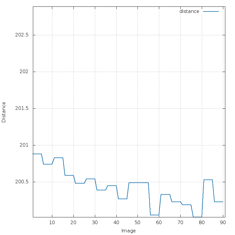
% cd 00
% ls -ltra
% ls -ltra *.png
% display distance.png
...

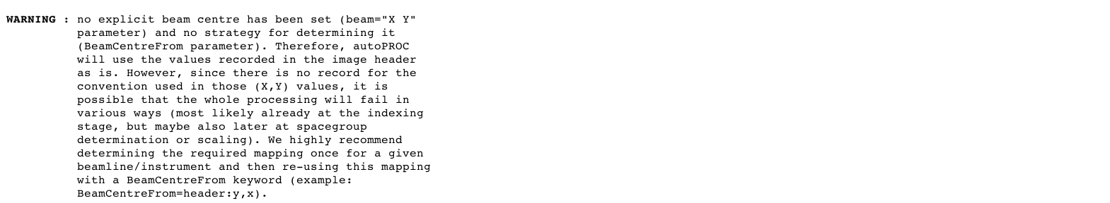
Since the specification of the beam centre (or detector) is a crucial part, some information is given:

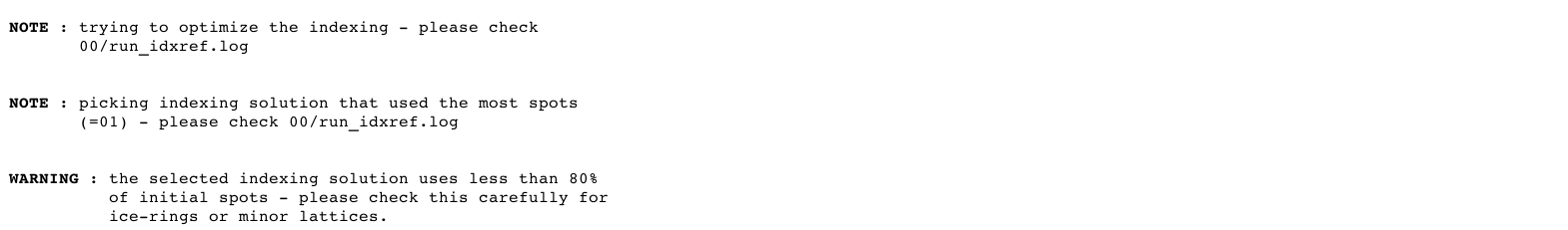
It seems there is some problem regarding indexing - autoPROC enters the so-called "iterative indexing" mode:

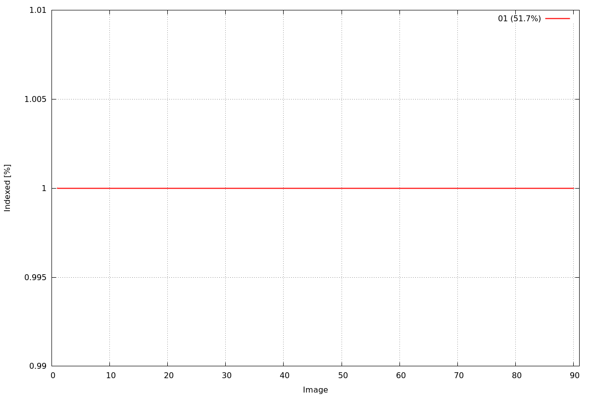
Remember, we would always like to index all spots on the images - anything not indexed is something to look at:

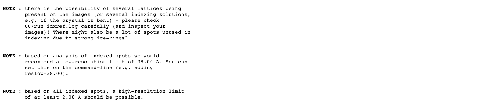The above rough resolution limits are based on spots - where a spot is most often much stronger than a still useful reflection: so the high-resolution limit is probably conservative.

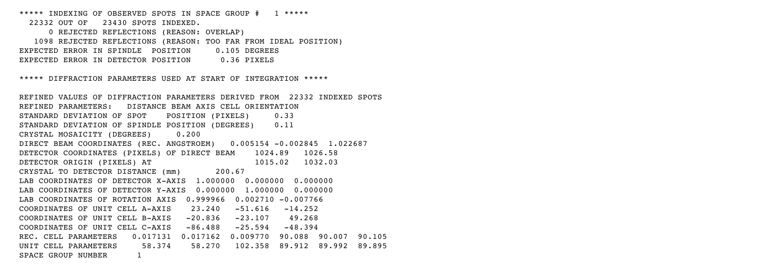
By default, the initial indexing is done in P1. Hopefully we reach a good indexing solution with small errors:

The first list of possible indexing solutions for different lattices already give an indication of the spacegroup:

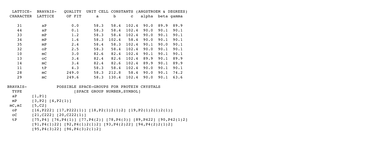After the initial integration (in P1) we use POINTLESS to decide on most likely spacegroup:

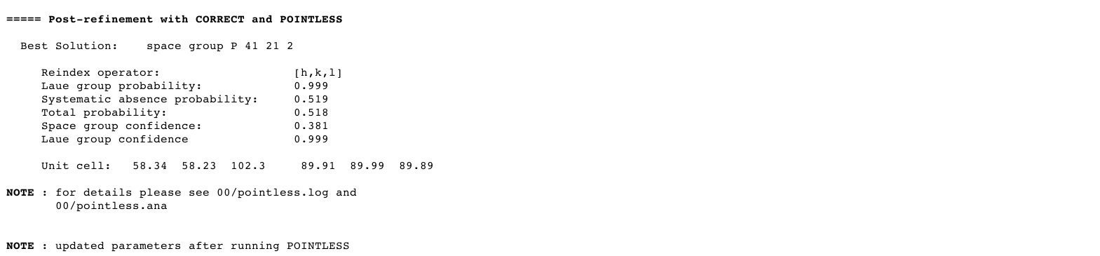It is always a good idea to check the above analysis very carefully: are all symmetries defined with the same probability? Was there enough data available to make such a crucial decision about spacegroup?

A quick analysis of data quality using the chosen spacegroup can eg already give an indication of anomalous signal:

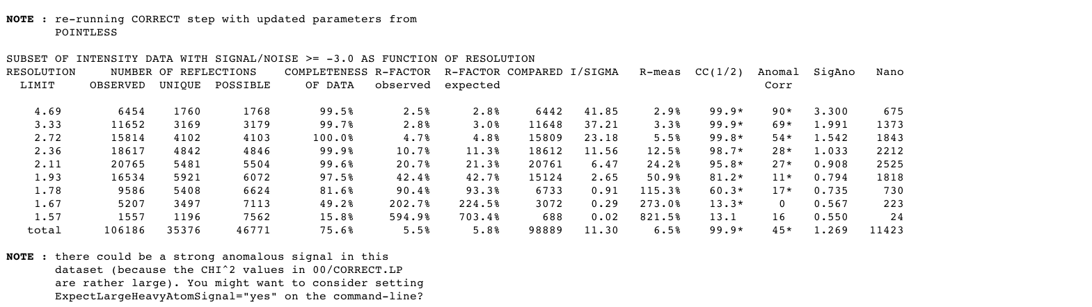Another round of integration is done, now in the higher symmetry spacegroup:

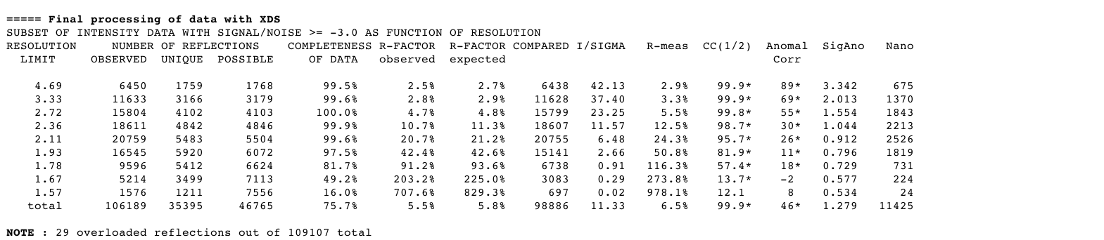We follow this with a scaling cycle using AIMLESS:

resulting in a "table 1" set of statistics:

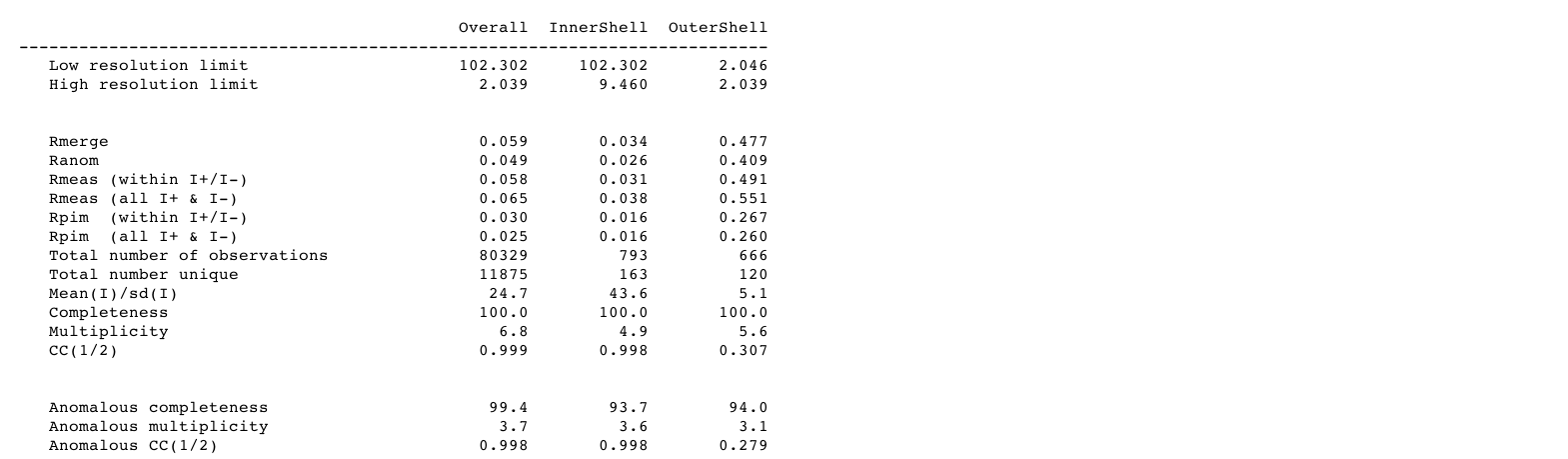In case of severe anisotropy, AIMLESS will give some indication of the problem:

Finally, we get a processed reflection file and the required section for structure deposition (REMARK 200):

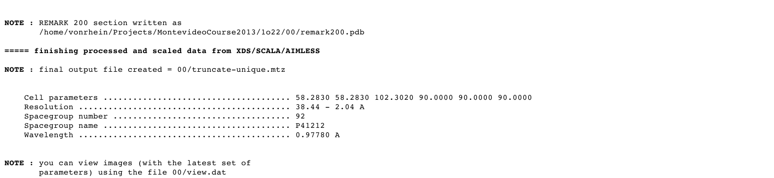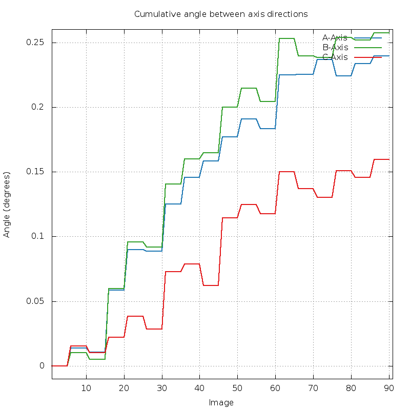
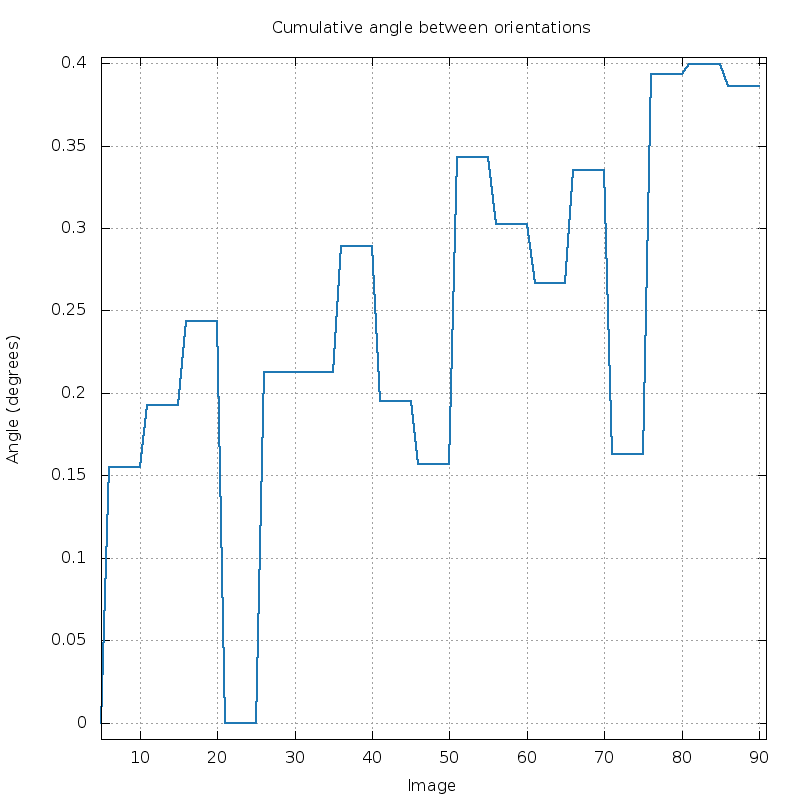
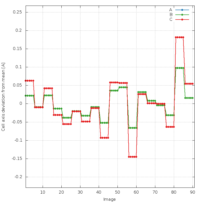
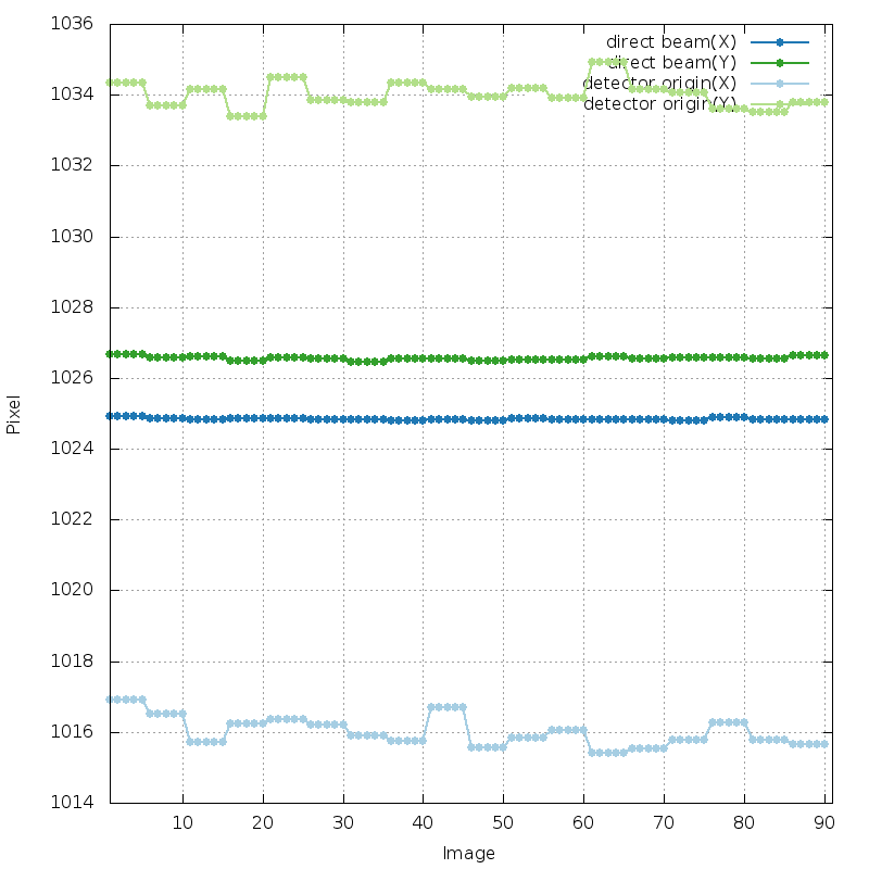
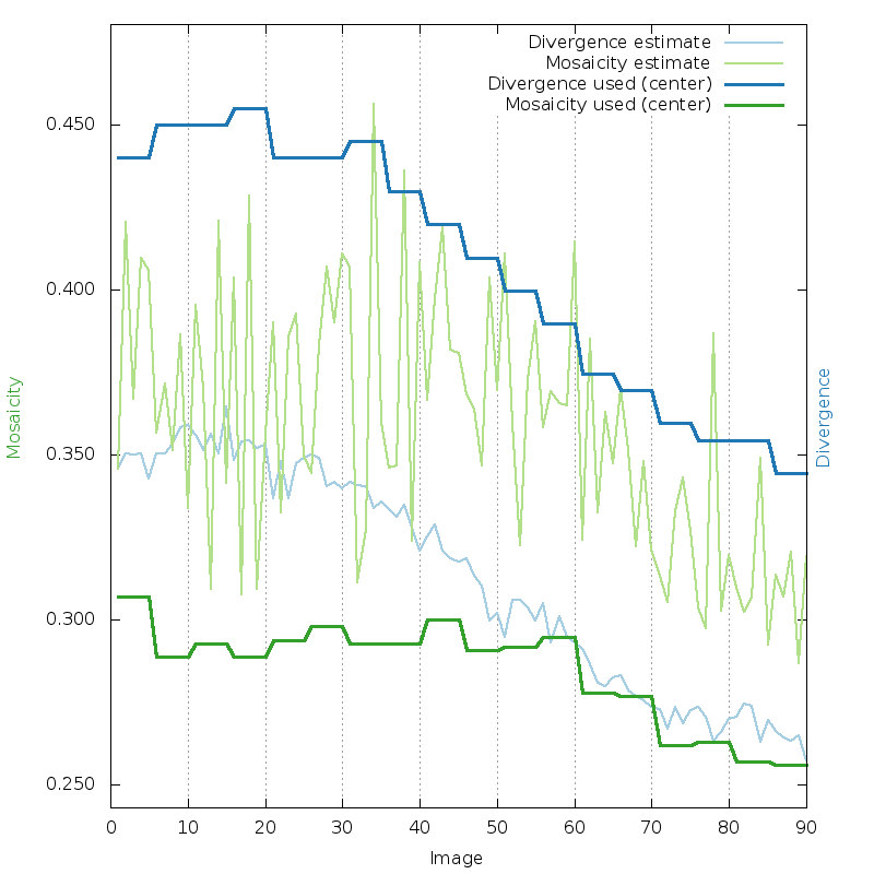
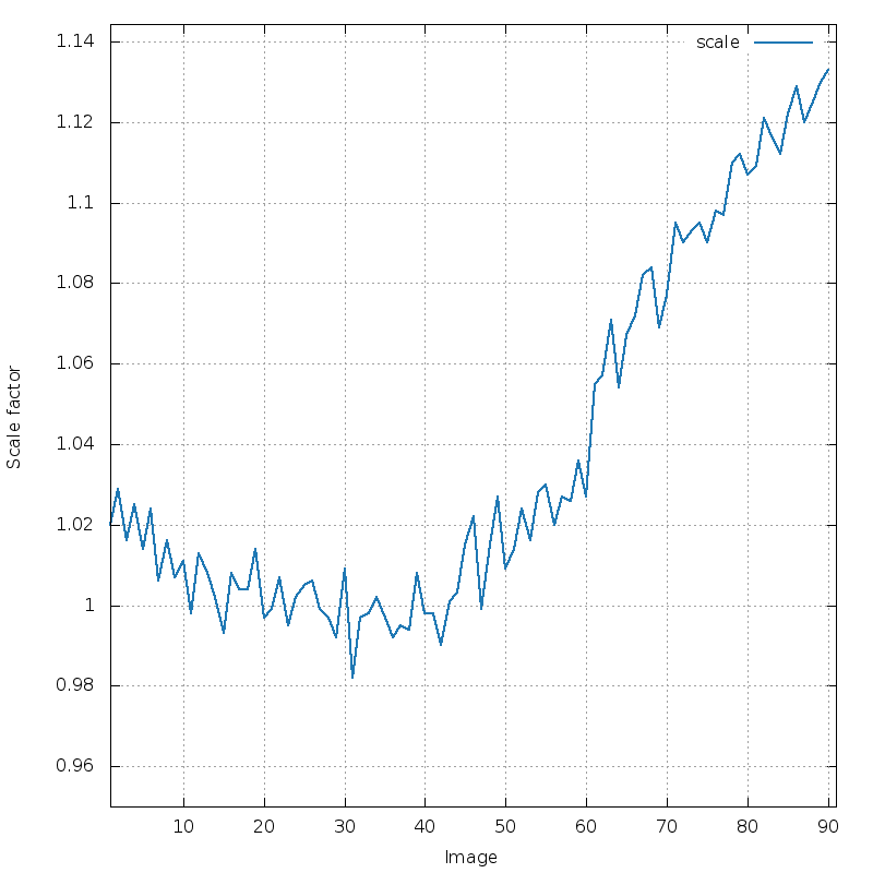
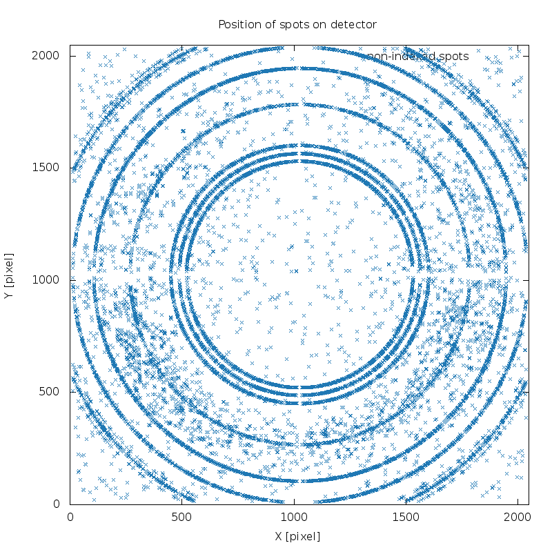
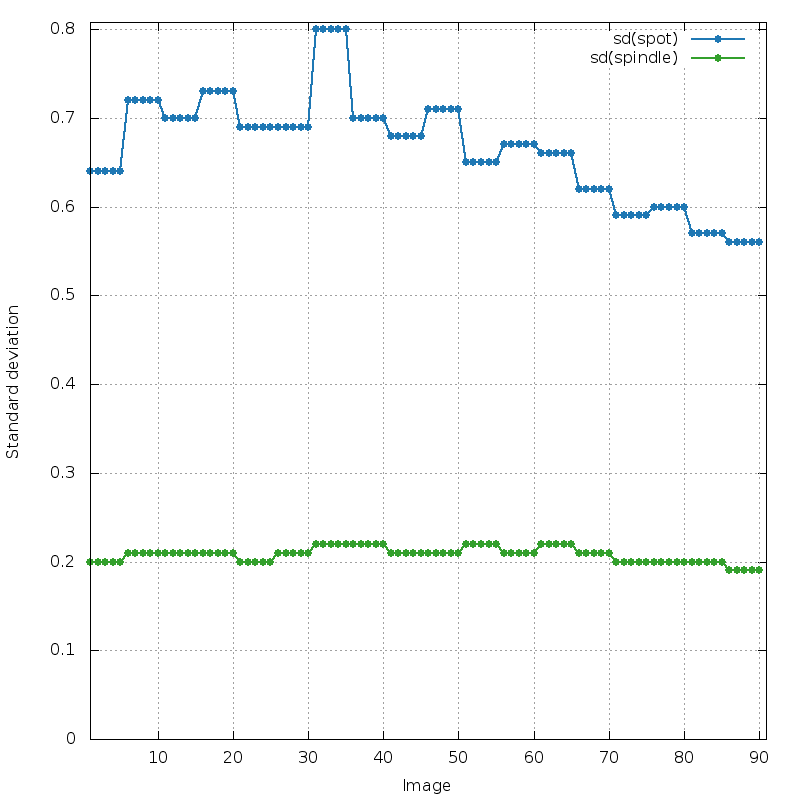
You should also have a look at the various graphs (PNG files) eg. with

% display 00/*.png

What do they show? Anything interesting in those images? What shape would we expect and where do we get deviations from that expectaions?

You should also look at the scaling logfile using:

% loggraph 00/aimless.log

---

own data

Make sure you know where to find documentation and help online:

• autoPROC reference card: handouts are also available in print.
• Wikis:
• autoPROC
• SHARP/autoSHARP
• BUSTER
• and

       % process -h
       % refine -h

autoPROC (data processing)

Ideally just running e.g.

% process -d 01 | tee 01.lis

in your directory with the images should be enough. However, often it is necessary to provide some additional, non-default parameters to describe the beamline/instrument - see here for some more information.

If you have potentially difficult data, you could also try and run with

% process -M LowResOrTricky -d 02 | tee 02.lis

Please see the autoPROC reference card (on the course moodle site) and the autoPROC wiki for more help - or type

% process -h
% process -M list

---

Original page: April 2013, Clemens Vonrhein