Most of the explicit commands given throughout this tutorial assume a sh-like shell (bash, zsh, ksh etc). There are given in the form
% ls -l
If you are using tcsh (or csh), please adapt the examples accordingly in case there is a sntax difference.
~/GlobalPhasing/data/autoproc/3isy/infl
~/GlobalPhasing/data/autoproc/3isy/hrem
            Distance: 275.01
            BeamCenter X: 162.5
            BeamCenter Y: 162.5
            PhiDelta: 1.00
            PhiStart: 322.00
            FrameNumber start: 1
            FrameNumber end: 90
            Distance: 275.01
            BeamCenter X: 162.5
            BeamCenter Y: 162.5
            PhiDelta: 1.00
            PhiStart: 322.00
            FrameNumber start: 1
            FrameNumber end: 90
Ideally one should run this tutorial in an empty directory, e.g. with
% mkdir -p ~/3isy/autoPROC
% cd ~/3isy/autoPROC
Then we want to copy the images over, which can be done with
% ln -s ~/GlobalPhasing/data/autoproc/3isy/*/*mccd .
Note: jobs will run faster if the images are located on a local disk. Often, a users HOME directory is a network filesystem - so this might not be a good location (not only sloing this autoPROC job down, but also everyone else that is using that same disk). If there is a large local disk available (e.g. /scratch or /tmp), we would recommend unpacking the files into a directory on that local filesystem. One can check the available size e.g. with
% df -h /tmp
% df -h /scratch
Once we have the images, we can have a closer look at some basic information about them. For that we have the tool imginfo that reads the header information and produces a consistent output format for those items:
% imginfo *001.mccd
which returns
################# File = 120482_1_E1_001.mccd

>>> Image format detected as MARCCD

===== Header information:
date                                = 14 May 2009 02:15:38
exposure time             [seconds] = 2.000
distance                       [mm] = 275.006
wavelength                      [A] = 0.979340
Phi-angle (start, end)     [degree] = 322.000 323.000
Oscillation-angle in Phi   [degree] = 1.000
Omega-angle                [degree] = 0.000
Chi-angle                  [degree] = 0.000
2-Theta angle              [degree] = 0.000
Pixel size in X                [mm] = 0.079346
Pixel size in Y                [mm] = 0.079346
Number of pixels in X               = 4096
Number of pixels in Y               = 4096
Beam centre in X               [mm] = 162.500
Beam centre in X            [pixel] = 2047.992
Beam centre in Y               [mm] = 162.500
Beam centre in Y            [pixel] = 2047.992
Overload value                      = 65535

################# File = 120482_1_E2_001.mccd

>>> Image format detected as MARCCD

===== Header information:
date                                = 14 May 2009 02:21:51
exposure time             [seconds] = 2.000
distance                       [mm] = 275.006
wavelength                      [A] = 0.911620
Phi-angle (start, end)     [degree] = 322.000 323.000
Oscillation-angle in Phi   [degree] = 1.000
Omega-angle                [degree] = 0.000
Chi-angle                  [degree] = 0.000
2-Theta angle              [degree] = 0.000
Pixel size in X                [mm] = 0.079346
Pixel size in Y                [mm] = 0.079346
Number of pixels in X               = 4096
Number of pixels in Y               = 4096
Beam centre in X               [mm] = 162.500
Beam centre in X            [pixel] = 2047.992
Beam centre in Y               [mm] = 162.500
Beam centre in Y            [pixel] = 2047.992
Overload value                      = 65535
What we can see from that:
To get a detailed record of the sequence of data-collection we need to use the timestamp in the image header (the timestamp on the file could easily be messed up through copying):
% imginfo -v *.mccd | awk '/File/{f=$NF}/Epoch/{print f,$NF}' | sort -n -k 2
which returns the list of images sorted by time (epoch, i.e. seconds since 01.01.1970). A slightly shortened output looks like this:
120482_1_E1_001.mccd 1242267338
120482_1_E1_002.mccd 1242267349
120482_1_E1_003.mccd 1242267360
...
120482_1_E1_028.mccd 1242267637
120482_1_E1_029.mccd 1242267648
120482_1_E1_030.mccd 1242267659
120482_1_E2_001.mccd 1242267711
120482_1_E2_002.mccd 1242267723
120482_1_E2_003.mccd 1242267736
...
120482_1_E2_028.mccd 1242268057
120482_1_E2_029.mccd 1242268070
120482_1_E2_030.mccd 1242268083
120482_1_E1_031.mccd 1242268133
...
120482_1_E1_060.mccd 1242268456
120482_1_E2_031.mccd 1242268507
...
120482_1_E2_060.mccd 1242268875
120482_1_E1_061.mccd 1242268926
...
120482_1_E1_090.mccd 1242269249
120482_1_E2_061.mccd 1242269302
...
120482_1_E2_090.mccd 1242269668
This shows nicely the collection pattern for an interleaved wavelength scan.
The easiest is to run a command like
% process -d 01 >01.lis 2>&1 # sh/ksh/bash/zsh
or (if one uses csh/tcsh as shell)
% process -d 01 >& 01.lis # csh/tcsh
The above example (with all default settings) assumes that the images are in the same directory the 'process' command is started in. If this is not the case, two mechanisms are provided:
% process -I /dir/where/images/are -d 01 > 01.lis 2>&1
% process -Id lowRes,/data/images1,lyso_###.img,1,90 -Id highRes,/data/images2,lyso_high_###.img,1,180 -d 01 > 01.lis 2>&1
The basic assumption for a single autoPROC run (using the process command) is that all images used in that run have a clearly defined relation in terms of orientation. That means that those cases work:
whereas those wont't:
Furthermore, the relation between different scans need to be clearly defined through
Running
% process -d 01 > 01.lis 2>&1
will process all found images (in the current directory) with a reasonable set of defaults (we hope). There are two modifications that might be of interest:
% process -M fast -d 02 > 02.lis 2>&1
% process -M automatic -d 03 > 03.lis 2>&1
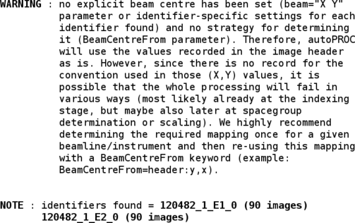
The first thing you'll see is some information about the way autoPROC was run (list of command-line arguments). There is a fairly lengthy paragraph about the beam centre: since this is very often the main reason for a failing processing run, it is explicitely mentioned here again.
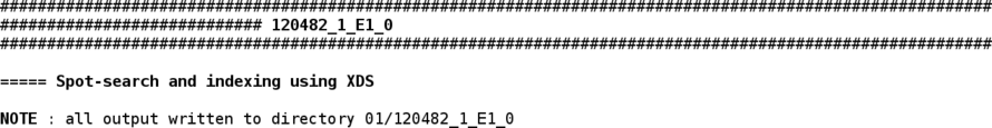
A list of found scans is presented (image identifiers and range of images that make up each scan). In this example here, only one scan is present (peak wavelength of a Se-MET MAD experiment).
The first step consists of finding spots on a set of images. The default is to search for spots on all images available. Although this might seem excessive (and often is required for getting a successful indexing), there are various analysis steps that work much more reliably if a larger number of images were used for spot search. These include:
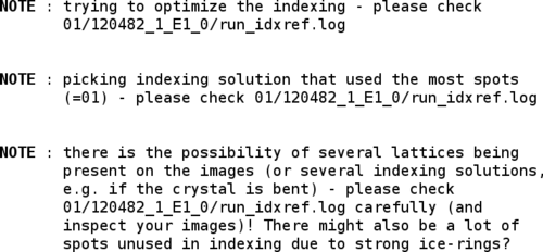
In this case, autoPROC decided that the initial indexing solution was not quite good enough to be used directly - mainly because the solution doesn't predict all of the found spots. A procedure for improving that initial solution will be used (run_idxref tool), which can e.g. detect multiple lattices or ice-rings.
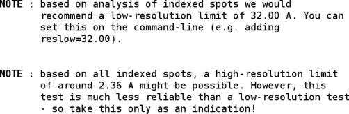
Using the list of indexed spots, some predictions of likely low- and high-resolution limits can be made as well.
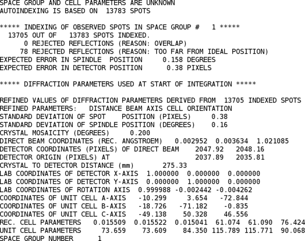
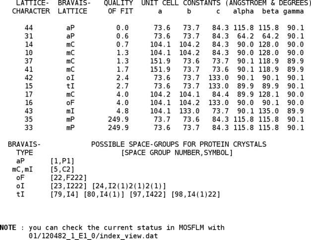
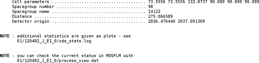
One can already see, that P1 might not be the finally correct spacegroup (two cell axes are nearly identical and the angles are very close to 90 degree). However, to do a final assignment of the most likely space group it is better to have a full set of integrated intensities available - so the following integration is till run in spacegroup P1.
If the user is very confident about the space group and cell, autoPROC can be run with
% process cell="74 74 132 90 90 90" symm="I4122" -d 02 > 02.lis 2>&1
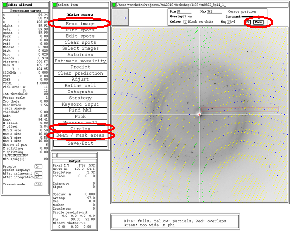
At this point, a little text file is prepared to allow visualisation of the current orientation matrix (and therefore predictions) using MOSFLM.
This can be very useful to check if everything is working correctly - especially since XDS doesn't have a viewer to show (and modify) predictions:
% ipmosflm < 01/120482_1_E1_0/index_view.dat
This will start the (old) MOSFLM interface - so make sure to have a binary that still supports this interface.
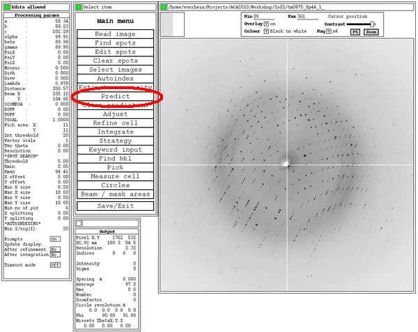
After hitting the 'Predict' button, the predictions given the current orientation matrix are shown: these should superimpose on actual spots . Ideally, all spots should have a prediction box around them: this depends on an accurate estimate of mosaicity though. After the initial indexing this value isn't yet available, but can be estimated from within MOSFLM:
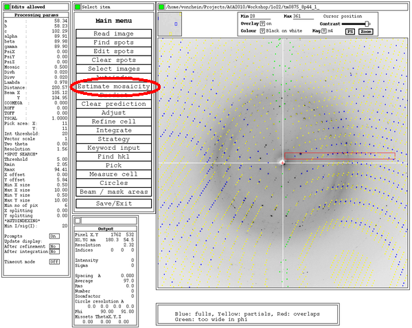
Some additional tools within this MOSFLM interface could be useful, e.g.
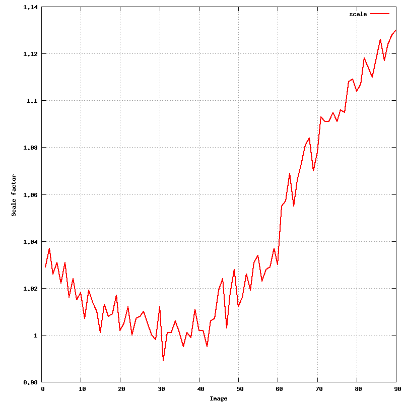
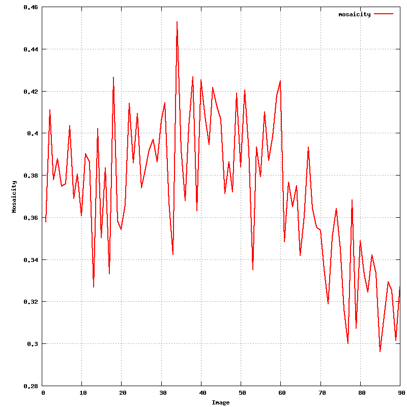
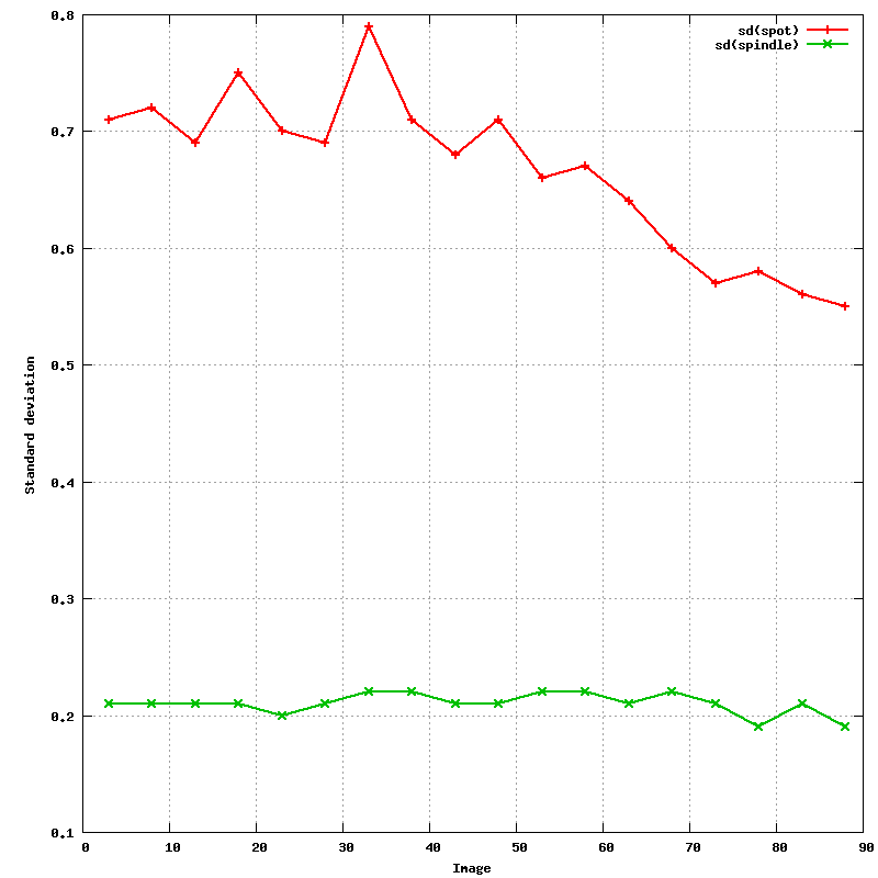
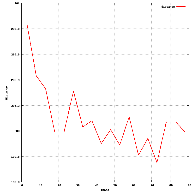
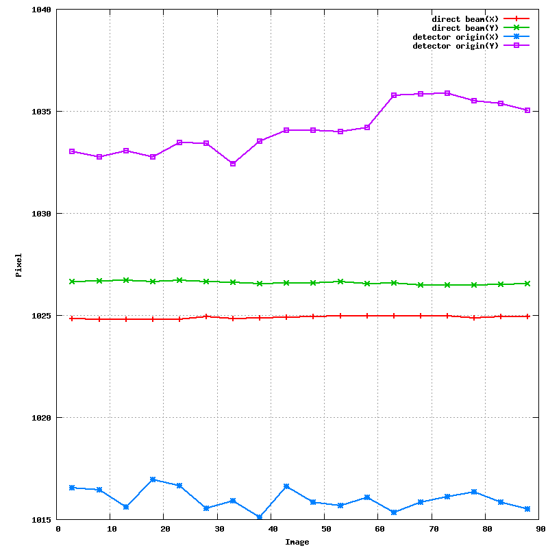
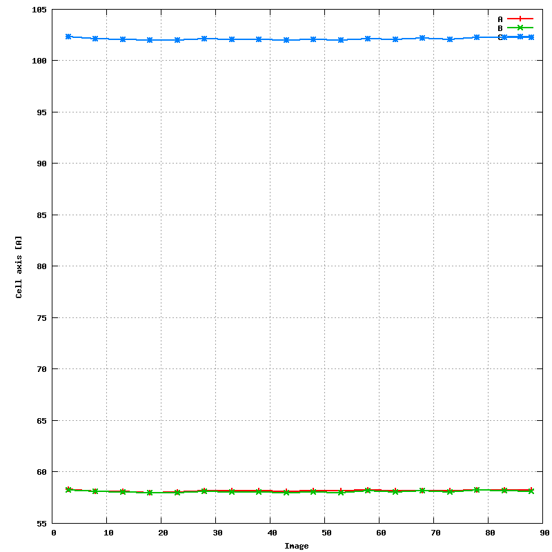
After the first integration (by default in P1), some additional plots are available for inspection:
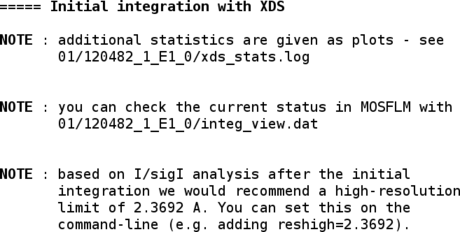
% display 01/120482_1_E1_0/*.png
An updated file for visualisation using MOSFLM is also written.
Since by default the initial integration was done in P1, POINTLESS is now used to determine the most likely space group:
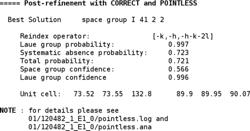
This step can obviously not analyse screw axes if no (or insufficient) reflections along that axis were collected. Also, a distinction between enantiomeric space groups (P41212 versus P43212) is not possible at that stage - for that the structure solution step is usually required (density modification in case of experimental phasing or molecular replacement in both possibilities).
Using the determined space group, the final post-refinement step is repeated:
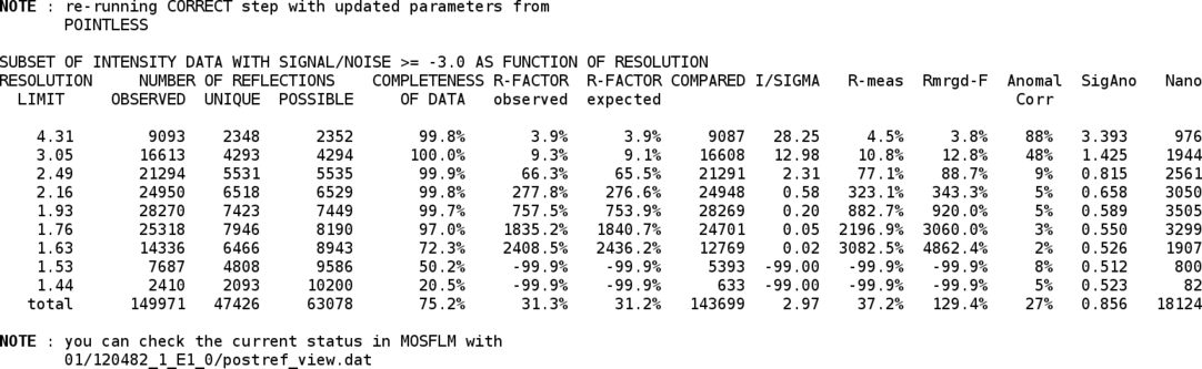
Now that the (hopefully) correct space group is know, the integration is repeated with these settings. At the end an updated table of statistics, a summary and an updated visualisation file are produced:
Now that a set of integrated intensities is available, they need to be scaled and merged with an appropriate high-resolution cut being applied. For that we use the SCALA program (through the "aP_scale" tool). The scaling step can also be run by hand using the "aP_scale" tool - for more help just run
% aP_scale -h
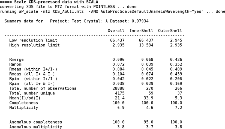
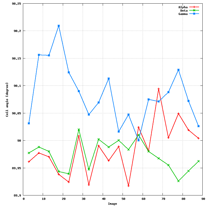
To see some detailed information about the scaling step, the CCP4 "loggraph" utility can be used - e.g.
% loggraph 01/120482_1_E1_0/scala.log
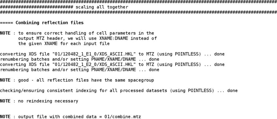
Since this dataset consists of two wavelengths, the same process as above is now repeated for the second wavelengths. At the end, the reflections from both scans are combined:
The two wavlengths are then scaled together (improving scale determination as well as outlier detection):
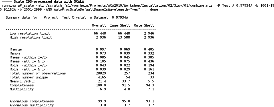
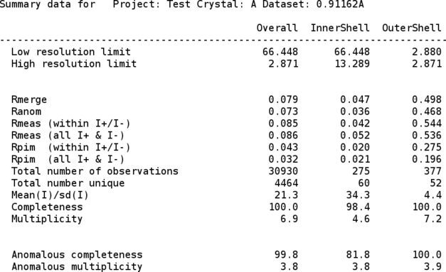
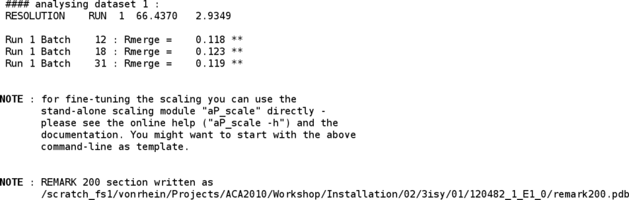
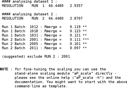
Some additional information regarding the different runs/scans (e.g. images/batches that might have slightly higher Rmerge values) is also given:
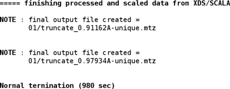
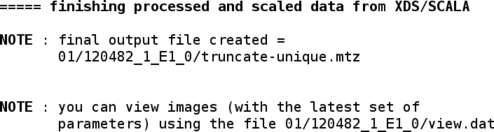
The merged intensities are then converted into amplitudes (and anomalous differences) with the CCP4 "truncate" program:
Details can be seen using
% loggraph 01/truncate_0.91162A.log
% loggraph 01/truncate_0.97934A.log
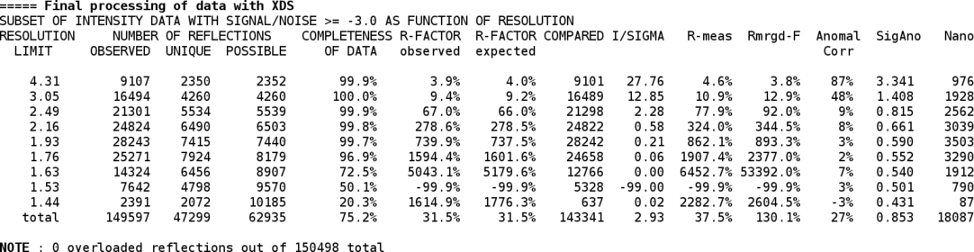
The final set of results will consist of