What SHARP can do

Contents

• Phasing scenarios
  • Introduction
  • SAD
  • SIR(AS)
  • MAD
  • MIRAS
  • MAD + native
  • Others
• Residual maps
• Density modification
• External phase information

Introduction

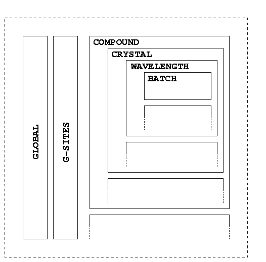
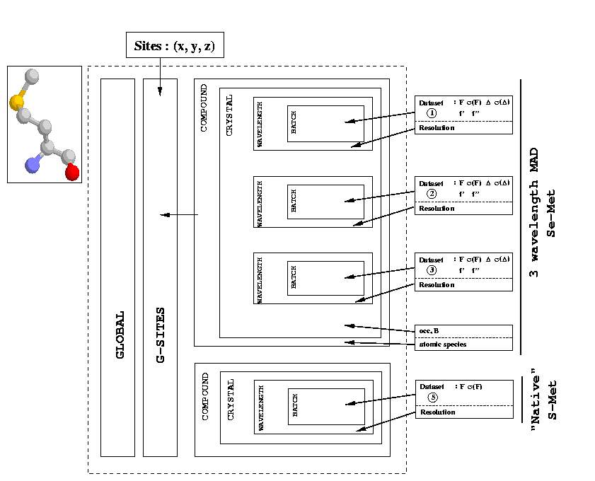
We will use a simplified description of the SHARP hierarchy as well (which is similar to what you're going to see on the left hand side of your SIN file editor). The notation of this hierarchy (tree structure) is:

	C-<i>	Compound <i>
	X-<j>	Crystal <j>
	W-<k>	Wavelength <k>
	B-<l>	Batch <l>

It might be a good idea to go through all of the presented examples here, even if you're going to do MAD right away. The ordering is so as to show you the buildup of more complicated phasing scenarios starting from the simplest case. This can help you in understanding the hierarchical structure of the SHARP input.

SAD

The nice thing about SAD is that you don't have to consider non-isomorphism between different crystals/datasets. If you have significant radiation damage during data collection of a MAD experiment it might be beneficial to start with a simple SAD refinement - using the first (peak?) wavelength only. Once this refinement has stabilised you can add additional wavelengths to see if the increased non-isomorphism doesn't outweigh the additional accuracy that you should be getting by using multiple wavelengths.

You don't necessarily need to travel to a synchrotron to collect a good dataset for SAD: some elements (e.g. Fe) have a nice anomalous signal at Cu K_a wavelength. For other elements data collection at a synchrotron source (with tunable wavelengths) is obviously more appropriate.

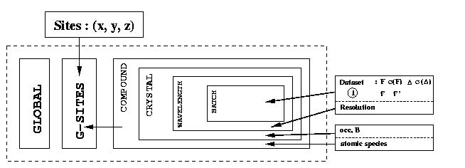
The simple layout will look like this:

	C-1
	X-1
	W-1	reference
	B-1

You can estimate the scale factor K for your data (putting it on roughly absolute scale if your atomic composition is correct). You can't estimate the temperature scale factor B. Additionally, you can't refine any of these two parameters.

Since we only have a single wavelength there are - obviously - no isomorphous/dispersive differences available. Therefore, the only non-isomorphism parameters one can refine are based on the anomalous differences. This is generally true for the reference dataset: there are no isomorphous/dispersive for the reference dataset!

Your MTZ file will contain the columns

	FMID	amplitude: F
	SMID	standard deviation of FMID: sigma(F)
	DANO	anomalous difference: F+ - F-
	SANO	standard deviation of DANO: sigma(F+ - F-)
	ISYM	flag to specify which of either F+ or F- was
		measured for an acentric reflection if no anomalous data
		is present.

SIR(AS)

	C-1
	X-1
	W-1	reference
	B-1
	C-2
	X-1
	W-1
	B-1

As reference you want to use your best dataset: this is quite often your native - but it doesn't have to! The important point is, that your MTZ file should have the cell parameters of your reference data set. This is necessary since all G-SITES are defined within this cell that is assumed to have zero non-isomorphism.

For the reference dataset the same restrictions about scaling and non-isomorphism parameters apply as for the SAD case. For the second compound, however, one can now not only estimate scale factors (multiplier K and temperature factor B) but also refine these. Furthermore, since any non-reference dataset has per definition isomorphous/dispersive differences (to the reference) non-isomorphism parameters based on these differences can be refined. If anomalous differences are present, non-isomorphism parameters based on these can be refined.

In cases where only low resolution (below 3 Å) is available, the temperature factor like parameters (temperature scale factor and both global non-isomorphism parameters) might not be well determined. In these cases it might be helpful to switch their refinement off (and set these to zero values).

Your MTZ file will contain the columns

	FMIDnat	native data
	SMIDnat
	FMIDder
	SMIDder
	DANOder	derivative data
	SANOder
	ISYMder

MAD

	C-1
	X-1
	W-1	reference
	B-1
	W-2
	B-1
	W-3
	B-1

The "branching" now happens at the Wavelength level. This has the (intended) side effect, that all parameters at the Compound and Crystal level are shared by the three wavelengths: all wavelengths have heavy atoms with identical coordinates x, y and z (G-SITES), chemical type (C-SITES), occupancy and temperature factor (T-SITES).

One of the most important parameters for this type of calculation are the scattering factors f' and f'' for each wavelength. Ideally, these should come from a fluorescence scan on the same or (eg in the case of Se-MAD) a very similar crystal. If you haven't got this information, your second best bet is probably to use some kind of "standard" values - usually available from knowledgeable colleagues or the beam-line personnel. This seems to work quite well in standard cases like Se-MAD. If even that is not possible, one note of advice: tabulated or calculated values (eg by the CCP4 program CROSSEC tend to be correct when far away from the edge. But: at or close to the edge these values can be very wrong.

But in general, a fluorescence scan will be available - otherwise how did you find your edge in the first place?

Your MTZ file will contain the columns

	FMIDpk
	SMIDpk
	DANOpk	peak wavelength
	SANOpk
	ISYMpk
	FMIDinf
	SMIDinf
	DANOinf	inflection point wavelength
	SANOinf
	ISYMinf
	FMIDhrm
	SMIDhrm
	DANOhrm	high energy remote wavelength
	SANOhrm
	ISYMhrm

It is recommended to input the wavelengths in the same order they were collected: usually peak -> inflection -> remote. With modern synchrotron sources the effects of radiation damage even for cry-cooled crystals can't be underestimated. And we want the best dataset as reference. You might be able to see the effects of radiation damage through an increase in non-isomorphism parameters during the refinement.

MIR(AS)

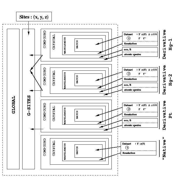
	C-1
	X-1
	W-1	reference
	B-1
	C-2
	X-1
	W-1
	B-1
	C-3
	X-1
	W-1
	B-1

One word about choice of reference: if your two derivatives are quite similar (eg both are Hg soaks that probably have quite a few sites in common) it is probably better to pick one of these two compounds as reference. Why that? The two derivatives might have very low non-isomorphism between them - or the same kind of non-isomorphism relative to your native dataset, which is the same. If you pick the native as a reference, compounds 2 and 3 will have similar, correlated non-isomorphism. The treatment of non-isomorphism in SHARP (for now) assumes that all non-isomorphism is un-correlated. Although some correlation might not be totally avoidable, it can make a big difference to the quality of the final phases to take some care when picking a reference. A graphical example for 2 Hg soaks and one Pt soak can be found here.

Obviously, there might be some drawbacks: what if the derivative datasets are of much worse quality than the native? Or of lower completeness? The resolution range might be more restricted ... This has to be a case-by-case decision.

If you run autoSHARP in MIR(AS) mode (even only to do the initial data scaling and analysis) you will get several tables of R-factors that might help you spotting clusters of similar datasets/derivatives. You probably want to pick a member of one of these clusters as a reference.

MAD + native

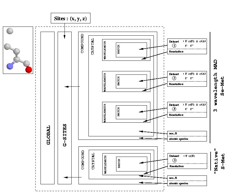
	C-1
	X-1
	W-1	reference
	B-1
	W-2
	B-1
	W-3
	B-1
	C-2
	X-1
	W-1
	B-1

What do we see? There are two things:

1. we defined two compounds since the native (S-Met) is chemically different from the 3 wavelength MAD (Se-Met).
2. we used the first MAD wavelength as a reference since we avoid correlated non-isomorphism this way.

1. define Se atoms in the 3 wavelength MAD datasets and S atoms in the native dataset (see picture).

   This assumes a protein with "holes" in the delta position of each methionine as the underlying structure. This has the disadvantage that the underlying structure is chemical nonsense and double the amount of heavy atom parameters have to be refined. The advantage is, that the definition of heavy atoms is logical and straightforward.

2. define Se-S atoms in the MAD datasets and nothing in the native (see picture).

   This assumes a protein with ordinary methionines (S-Met) as underlying structure. It has the disadvantage, that a special kind of heavy atom (Se-S) has to be defined. However, only one set of heavy atom parameters has to be refined.

Others

• Have a look at all your datasets to find how they differ chemically from each other - and what is common to all of them. This is needed to know where and how to define the heavy atom sites (see MAD + native discussion above).

• Try to assess the quality of each dataset: completeness, redundancy, I/sigma, R_merge, R_pim etc. It might be a good idea to give each dataset a very subjective ranking (brilliant -> good -> average -> poor -> disastrous). Don't expect brilliant phases from a disastrous dataset (although we're doing our best)!

• Collect all available information: f' and f'' values, resolution ranges, atomic composition (sequence), number of molecules in the asymmetric unit (Matthews parameter).

• Do not forget about any problems you had during data collection! If you're not sure about the space group try all possibilities.

• Start first with the best dataset(s) - especially in MIR(AS).

• Refine the parameters with the largest error first. This depends a lot on the specific case (eg if you have f' and f'' values from a very accurate fluorescence scan there is no need to refine these values).

Residual maps

• detecting minor sites
• detecting (and subsequently refining) anisotropic temperature factors on heavy atoms
• detecting split sites
• detecting overall anisotropy in your data (and distinguishing it from anisotropic temperature factors on heavy atoms)
• detecting wrong f'/f'' factors

Density modification

The various tools are:

• solvent flattening (actually solvent flipping)
• solvent flattening with various solvent contents to find the optimal solvent content
• detection of non-crystallographic symmetry (NCS) (for proper NCS of type C_n for now)
• use of solvent flattened phases to detect minor/additional sites through difference Fourier techniques.

There is also a direct connection to the ARP/wARP suite of programs. For further information please consult your original documentation for these programs.

The solvent flattening protocol(s) allows for a variety of parameters to be set. Although the defaults should give a reasonable result it might be worth to try slightly different values for maximum performance. All this is done through the Phase Improvement and Interpretation Control Panel which is accessible through the main log-file of a SHARP run (or from the Results page).

External phase information

If the phase information comes from another SHARP run these coefficients are already present in the output MTZ file (columns HLA, HLB, HLC and HLD in eden.mtz). To get these coefficients from a model (PDB file) one could use the CCP4 programs SFALL, SIGMAA and SFTOOLS.

Note 1 : it is important, that all external phase information is on the same origin as the heavy atom sites refined within SHARP.

Note 2 : strictly speaking, it is only valid to use this external phase information for calculation of the centroid structure factor (electron-density map) if this is independent phase information. Otherwise bias is introduced.