STARANISO
Anisotropy of the Diffraction Limit
and
Bayesian Estimation of Structure Amplitudes

|
| STARANISOAnisotropy of the Diffraction Limit
|
|
The statistical significance of the intensity data after merging is commonly expressed as either the value of the mean signal/noise ratio I/σ(I), or the half-dataset correlation coefficient CC½ [1], computed in spherical shells of reciprocal space. The statistical significance, in whatever form one chooses to express it, is used as a criterion for applying a diffraction cut-off to the reflection data that should match the diffraction limit as closely as possible. Clearly if the applied diffraction cut-off falls inside the diffraction limit, then useful data containing information about the structure will be lost; if it falls outside, then uninformative data will be kept.
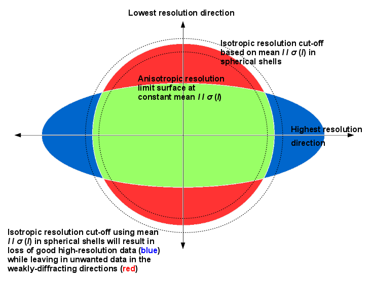 Since the diffraction limit may be anisotropic, in STARANISO the
locally-averaged value of I/σ(I), rather than its
spherical average, is used to define an anisotropic diffraction cut-off
- that is, a cut-off varying with direction in reciprocal space.
The boundary between statistically significant and insignificant data
therefore defines a surface, the anisotropic diffraction cut-off
surface (see diagram on right: click image to enlarge).
Since the diffraction limit may be anisotropic, in STARANISO the
locally-averaged value of I/σ(I), rather than its
spherical average, is used to define an anisotropic diffraction cut-off
- that is, a cut-off varying with direction in reciprocal space.
The boundary between statistically significant and insignificant data
therefore defines a surface, the anisotropic diffraction cut-off
surface (see diagram on right: click image to enlarge).
No assumption is made about the shape or orientation of the anisotropic diffraction cut-off surface, other than that it has at least the symmetry of the Laue class. This means that in orthorhombic and higher symmetry space groups the principal axes of the surface shape must coincide with the crystal axes. In monoclinic space groups only one of the principal axes of the surface shape is constrained to lie along a crystal axis, namely b, but there is no symmetry constraint on the second principal axis: it can lie anywhere in the ac plane since the choices of the a and c axes are completely arbitrary. Similarly, in triclinic space groups the choices of all three crystal axes are arbitrary so there are no symmetry constraints whatsoever on the directions of the principal axes of the surface shape.
Note that it is not assumed that the shape of the anisotropic cut-off surface is an ellipsoid (the contours in the figure below are clearly not ellipsoidal). The principal cause of distortion of the diffraction limit surface away from a perfect ellipsoid is the variation of the reflection redundancy through its effect on the σ(I) values of the merged data (i.e. inversely proportional to the square root of the redundancy), and therefore on the mean I / σ(I). The variation of redundancy in reciprocal space is largely arbitrary, being a consequence of both the experimental setup and the data collection strategy (whether a standard protocol or a deliberate user choice).
However, for the purposes of estimating the diffraction limit as a function of direction an ellipsoid is fitted to the anisotropic cut-off surface. Measured data with d* greater than the largest semi-axis length of the fitted ellipsoid are considered to be outside the anisotropic cut-off surface. Then all measured intensities (excluding any systematic absences) that fall inside this anisotropic cut-off surface are considered to be 'observed', that is they are included in the reflection statistics and are written to the reflection output file, while all those that fall outside are 'unobserved' and are not used further. Unmeasured data (except systematic absences) that fall inside the fitted ellipsoid (for example in a cusp) are deemed to be 'observable' (i.e. they had the potential to be observed if only they had been measured), whereas those unmeasured reflections falling outside the fitted ellipsoid are deemed to be 'unobservable' (i.e. not worth measuring).
 An example is the (h0l) zone of a diffraction pattern
shown on the right: the space group is C2 in the conventional IUCr
monoclinic setting with β nearest to 90o (β =
99o). The local mean value of I/σ(I)
is color-coded for each reflection within the limiting sphere of
measurement. Representing unmeasured reflections, pink points are 'unobservable' (i.e.
expected to be unobserved), whereas blue points are 'observable' (i.e.
expected to be observed had they been measured). Representing
measured reflections, red points
are unobserved data with their local mean
I/σ(I) falling below the default significance
threshold of 1.2 (a white point in the red region is an unobserved
reflection with individual intensity measured above 3 times its
own σ). The other colors for measured and
observed reflections represent successively higher values of the
local mean I/σ(I) in increasing value: orange,
yellow, green, cyan, magenta, white.
An example is the (h0l) zone of a diffraction pattern
shown on the right: the space group is C2 in the conventional IUCr
monoclinic setting with β nearest to 90o (β =
99o). The local mean value of I/σ(I)
is color-coded for each reflection within the limiting sphere of
measurement. Representing unmeasured reflections, pink points are 'unobservable' (i.e.
expected to be unobserved), whereas blue points are 'observable' (i.e.
expected to be observed had they been measured). Representing
measured reflections, red points
are unobserved data with their local mean
I/σ(I) falling below the default significance
threshold of 1.2 (a white point in the red region is an unobserved
reflection with individual intensity measured above 3 times its
own σ). The other colors for measured and
observed reflections represent successively higher values of the
local mean I/σ(I) in increasing value: orange,
yellow, green, cyan, magenta, white.
The data are clearly highly anisotropic with the principal directions of the anisotropy in this case lying along the [-1,0,1], [0,1,0] and [1,0,1] directions. STARANISO deals optimally with this situation by truncating only the red regions (i.e. also removing the embedded white points). Incidentally, it can be seen that there is some truncation of significant data (orange points) by the edges of the detector in the top left and bottom right quadrants shown by the 'caps' of unmeasured blue points inside the fitted ellipsoid (data courtesy of Esther Ortega and Jose M. de Pereda at the Instituto de Biología Molecular y Celular del Cancer, Salamanca, Spain).
T(s) = exp(-4π2sTUs)
The diffraction image on the right is the same as the one above but
shows instead the ellipsoidal contours of the Debye-Waller
factors. The pink, blue and red
points have the same meaning as above; the other colors represent
increasing values of the Debye-Waller factor towards the center of the
pattern.

The inverse of the square root of the Debye-Waller factor is applied as an anisotropic correction factor to the amplitudes after Bayesian estimation from the measured intensities and their standard uncertainties. The method is that of French & Wilson [6], except that it uses an anisotropic prior distribution of the expected intensity, calculated from the Debye-Waller factor for each reflection, instead of the isotropic prior originally proposed. The anisotropic correction factor is adjusted by subtracting the smallest eigenvalue of the overall anisotropic displacement tensor U from the diagonal elements of U. Thus, no correction is applied in the direction of the eigenvector corresponding to the smallest eigenvalue of U (i.e. the direction of least mean-square displacement), and a multiplicative correction factor > 1 is applied in all other directions. The corrected amplitudes therefore decay isotropically at high values of d*, at the same rate as those in the direction of strongest diffraction. In other words, the data in the weaker-diffracting directions are sharpened so as to decay at the same rate as those in the strongest-diffracting one, with the latter remaining unchanged.
[1] Karplus, P.A. & Diederichs, K. (2012) "Linking crystallographic data with model quality. " Science 336, 1030-3.
[2] Popov, A.N. & Bourenkov, G.P. (2003) "Choice of data-collection parameters based on statistical modelling". Acta Cryst. D59, 1145-53.
[3] Wilson, A.J.C. (1987) "Treatment of enhanced zones and rows in normalizing intensities." Acta Cryst. A43, 250-2.
[4] Debye, P. (1913) "Interferenz von Röntgenstrahlen und Wärmebewegung." Annalen der Physik 348, 49–92.
[5] Waller, I. (1923) "Zur Frage der Einwirkung der Wärmebewegung auf die Interferenz von Röntgenstrahlen." Zeitschrift für Physik A17, 398–408.
[6] French, S. & Wilson, K.S. (1978) "On the treatment of negative
intensity observations." Acta Cryst. A34, 517-525, and
"Bayesian
treatment of negative intensity measurements in crystallography"
(2012, unpublished).