|
From the session website: We often encounter datasets that include weak experimental phases that we must depend on in order to solve our structures. The following two datasets are examples of data collected for the purposes of solving structures by Single-wavelength Anomalous Diffraction (SAD) phasing. The anomalous signal is present, but weak, and therefore care must be taken to preserve the anomalous signal for phasing. This demonstration will educate the user on how to preserve the anomalous differences in a dataset. |
Content:
Running
% find_images
shows us two datasets of 360 images each: ACA10_AF1382_1.0001 to ACA10_AF1382_1.0360 and ACA10_AF1382_2.0001 to ACA10_AF1382_2.0360. To get some more detail, we run
% imginfo ACA10_AF1382_1.0001 ACA10_AF1382_2.0001
that gives
################# File = ACA10_AF1382_1.0001

>>> Image format detected as MARCCD

===== Header information:
date                                = 13 Jun 2007 13:58:49
exposure time             [seconds] = 4.000
distance                       [mm] = 125.000
wavelength                      [A] = 1.900000
Phi-angle (start, end)     [degree] = 0.000 1.000
Oscillation-angle in Phi   [degree] = 1.000
Omega-angle                [degree] = 0.000
Chi-angle                  [degree] = 0.000
2-Theta angle              [degree] = 0.000
Pixel size in X                [mm] = 0.073242
Pixel size in Y                [mm] = 0.073242
Number of pixels in X               = 4096
Number of pixels in Y               = 4096
Beam centre in X               [mm] = 146.191
Beam centre in X            [pixel] = 1996.000
Beam centre in Y               [mm] = 148.535
Beam centre in Y            [pixel] = 2028.000
Overload value                      = 65535

################# File = ACA10_AF1382_2.0001

>>> Image format detected as MARCCD

===== Header information:
date                                = 13 Jun 2007 17:52:32
exposure time             [seconds] = 4.000
distance                       [mm] = 125.000
wavelength                      [A] = 1.900000
Phi-angle (start, end)     [degree] = 0.000 1.000
Oscillation-angle in Phi   [degree] = 1.000
Omega-angle                [degree] = 0.000
Chi-angle                  [degree] = 0.000
2-Theta angle              [degree] = 0.000
Pixel size in X                [mm] = 0.073242
Pixel size in Y                [mm] = 0.073242
Number of pixels in X               = 4096
Number of pixels in Y               = 4096
Beam centre in X               [mm] = 146.191
Beam centre in X            [pixel] = 1996.000
Beam centre in Y               [mm] = 148.535
Beam centre in Y            [pixel] = 2028.000
Overload value                      = 65535
So both were collected at the same wavelength, distance, osciallation angle and also starting at the same Phi angle. Maybe looking at the order the images were collected gives us some more information? With
% imgdate.sh -s * > img.lis
we get a listing of the collection time in file img.lis:
# sorted list of: file, Epoch, Date, seconds-to-previous
ACA10_AF1382_1.0001 1181743129  13 Jun 2007 13:58:49 0
...
ACA10_AF1382_1.0360 1181745227  13 Jun 2007 14:33:47 5
ACA10_AF1382_2.0001 1181757152  13 Jun 2007 17:52:32 11925
...
ACA10_AF1382_2.0360 1181758981  13 Jun 2007 18:23:01 5
So unless this was a very long coffee break, the gap of more than 3 hours between the first and the second dataset probably means that the crystal was taken off the instrument and later put back. Was the second dataset collected at the same spot of the crystal or on a fresh one? Does the instrument maintain the exact same orientation of the pin on the goniostat after unmounting/remounting - or is the starting value of zero for each scan a software setting that is unrelated to the actual hardware values? Or it is a different crystal altogether? Anyway, without the exact log of the actual data collection we won't know.
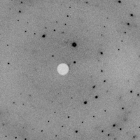
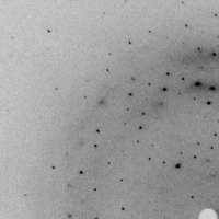
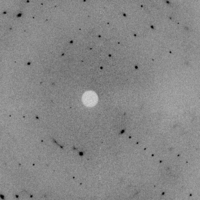
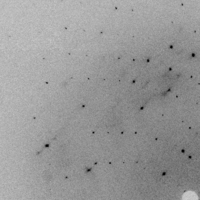
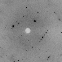
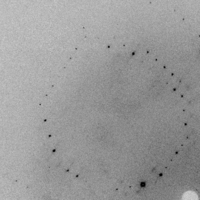
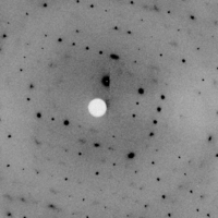
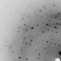
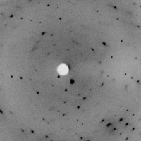
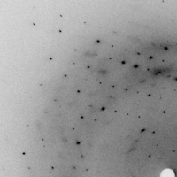
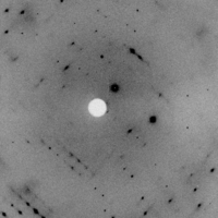
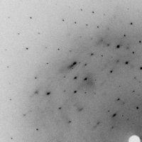
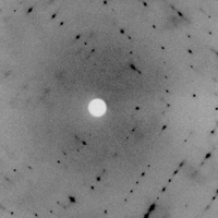
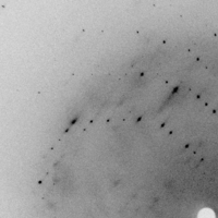
| Image | Full image | Central region | Upper-left |
| ACA10_AF1382_1.0001 |  |
 |
 |
| ACA10_AF1382_1.0031 |  |
 |
 |
| ACA10_AF1382_1.0061 |  |
 |
 |
| ACA10_AF1382_1.0091 |  |
 |
 |
| ACA10_AF1382_2.0001 |  |
 |
 |
| ACA10_AF1382_2.0031 |  |
 |
 |
| ACA10_AF1382_2.0061 |  |
 |
 |
| ACA10_AF1382_2.0091 |  |
 |
 |
Just running all defaults
% process -d 01 | tee 01.lis
gives
Summary data for   Project: Test Crystal: A Dataset: 1.900000

                                           Overall  InnerShell  OuterShell
---------------------------------------------------------------------------
  Low resolution limit                      19.251      19.251       2.317
  High resolution limit                      2.309      10.170       2.309

  Rmerge                                     0.052       0.048       0.595
  Ranom                                      0.051       0.046       0.574
  Rmeas (within I+/I-)                       0.053       0.048       0.595
  Rmeas (all I+ & I-)                        0.053       0.049       0.606
  Rpim  (within I+/I-)                       0.014       0.013       0.154
  Rpim  (all I+ & I-)                        0.010       0.011       0.112
  Total number of observations              148284        1498        1554
  Total number unique                         5267          61          53
  Mean(I)/sd(I)                               55.7        71.1         9.6
  Completeness                               100.0       100.0       100.0
  Multiplicity                                28.2        24.6        29.3

  Anomalous completeness                     100.0       100.0       100.0
  Anomalous multiplicity                      14.0        10.9        14.6
and the files
Can those already be used for solving the structure? See the autoSHARP tutorial.
Work in progress