Content:
Introduction
To include autoSHARP into an automated workflow (e.g. at a synchrotron), a command-line tool is provided to allow running of all autoSHARP scenarios like SAD, MAD, SIRAS or MIRAS - optionally including a partial model.
The only requirements are a current SHARP/autoSHARP installation and the environment variable SHARP_home pointing to that installation. This can be achieved using:
% setenv SHARP_home /where/ever/sharp
- or -
% export SHARP_home=/where/ever/sharp
The online help for the command-line tool is then accessible via
% $SHARP_home/bin/sharp/run_autoSHARP.sh -h
Output of above command:
============================================================================

Copyright (C) 2015 by Global Phasing Limited

          All rights reserved.

          This software is proprietary to and embodies the confidential
          technology of Global Phasing Limited (GPhL). Possession, use,
          duplication or dissemination of the software is authorised
          only pursuant to a valid written licence from GPhL.

----------------------------------------------------------------------------

Contact:  sharp-develop@GlobalPhasing.com

Program:  run_autoSHARP.sh   version  <2016-06-29 16:54:43>

============================================================================

USAGE: run_autoSHARP.sh [-h] [-seq <file>] [-nres <Nres>] [-faster] [-R <reslow> <reshigh>]\
       [-scaled] [-nobuild] [-spgr <SG-name>] [-id <ID>] [-pdb <file>] \
       -ha <hatom> [-nsit <nsit> [-sites <file>]] \
       [-wvl <lambda> [peak|infl|hrem|lrem] [<fp> <fdp>]|-nat] -sca|-mtz <file> ... \
       [-wvl <lambda> [peak|infl|hrem|lrem] [<fp> <fdp>]     ] -sca|-mtz <file>

       -h                           : this help message

       -seq <file>                  : ASCII sequence file (single letter code); FASTA or PIR

       -nres <Nres>                 : number of amino-acid residues per monomer

       -faster                      : running a faster (but potentially less accurate) path through
                                      the various stages. This flag can be given several times to go
                                      from the default rate of 5 (accurate) to 1 (fast).

       -R <reslow> <reshigh>        : (optional) explicit overall resolution limit to use;
                                      default is to use all data from input reflection files.

       -scaled                      : if several datasets are given, assume these are already
                                      scaled relative to each other. The default is to scale several
                                      datasets against the first one.

       -nobuild                     : the default is to attempt automatic building (and iterating this
                                      with density modification). This flag will switch that off - but
                                      still run the initial density-modification stage.

       -spgr <SG-name>              : (optional) space-group name; default is to take this from
                                      the reflection file.

       -id <ID>                     : (optional) run/job identifier; default="autoSHARP" (this will create
                                      a subdirectory of that name)

       -pdb <file>                  : (optional) model placed correctly in current data and SG

       -ha <hatom>                  : heavy-atom type (eg "Se", "Zn", "Os" ...)

       -nsit <nsit>                 : (optional) number of sites to expect; default based on input
                                      sequence (if heavy-atom is of type "Se" or "S")

       -sites <file>                : (optional) file (with .hatom extension) with a list of
                                      starting sites. One line per site in fractional coordinates,
                                      eg:

                                        ATOM Hg 0.3745 0.1277 0.9833

                                      This flag needs to be preceded by a "-nsit <nsit>" argument.

       -wvl <lambda> [peak|infl|hrem|lrem] [<fp> <fdp>]

                                      definition of dataset via wavelength (in Angstroem),
                                      an optional identifier and optional f'/f" values

       -nat                         : marking this as a SIR(AS)/MIR(AS) experiment: the next
                                      reflection file is expected to be the native data (and
                                      data given with the -wvl argument are derivatives)

       -sca <file>                  : merged (anomalous) SCALEPACK data file for current wavelength

       -mtz <file>                  : merged (anomalous) MTZ data file for current wavelength (containing
                                      amplitudes and anomalous differences)

NOTE:  several -wvl/-sca flag pairs can be given -
       and should be given for MAD or MIR(AS) experiments.

EXAMPLES:

   SAD:
        run_autoSHARP.sh -seq 1o22.pir -ha "Se" \
          -wvl 0.9778 peak -7 5 -sca 1o22_peak.sca

   MAD:
        run_autoSHARP.sh -seq 3isy.pir -ha "Se" \
          -wvl 0.97934 infl -11 3.3  -sca 3isy_aimless_0.97934A.sca \
          -wvl 0.91162 hrem -1.8 3.3 -sca 3isy_aimless_0.91162A.sca

   SIR(AS):
        run_autoSHARP.sh -seq 1GXT.pir -nat -mtz 1GXT_nat.mtz \
          -ha "Hg" -nsit 2 \
          -wvl 0.99970 peak -16 10 -mtz 1GXT_hg.mtz

   MIR(AS):
        run_autoSHARP.sh -seq 3zft.pir -nat -mtz 3zft_nat.mtz \
          -ha "Hg" -nsit 1 -wvl 1.54179 -mtz 3zfq_Hg.mtz \
          -ha "Ir" -nsit 2 -wvl 1.54179 -mtz 3zfr_Ir.mtz

   partial model:
        run_autoSHARP.sh -seq 3get.pir -ha "Se" \
          -pdb 3ffh_ala_MR.pdb \
          -wvl 0.9789 peak -8 4 -sca 3get.sca

   SAD with Ta6Br12 cluster:
        run_autoSHARP.sh -seq 4cv5.pir -ha "Ta6Br12:Ta" -nsit 1 \
          -wvl 1.25472 peak -mtz 4cv5.mtz
Typical usage
The input files for reflection data, sequence, model and heavy-atom positions are explained in detail in the autoSHARP manual. In most cases, one will use
- a merged SCALEPACK or MTZ file for reflections (e.g. from autoPROC)
- a simple ASCII sequence file
- (optionally) a PDB file with a partial model or initial MR solution
- a text file with externally determined heavy-atom positions (fractional coordinates)
We will now show some typical usage and explain the meaning of the command-line arguments at the same time.
SAD
4J8P from JCSG:
% run_autoSHARP.sh \
  -seq seq.pir -ha "Se" \
  -wvl 0.97858 peak -8.000 6.000  -mtz truncate.mtz \
  -id autoSHARP | tee autoSHARP.lis
Although we could run without a sequence file (and for RNA/DNA structures this would be the case anyway), it is always best to use the sequence of the monomer with the -seq flag. This will also simplify specifying the number of heavy-atom sites when using Se-MET or native sulfurs (-ha flag): in those cases the Met and Cys residues in the sequence file provide this number.
The -ha flag always needs to be given before the reflection files: it will define what heavy atoms are present in the subsequent reflection data.
If the heavy-atom is not instrinsic in the protein sequence (i.e. not Se-MET or native sulfur), the flag -nsit is required to specify the most likely number of heavy-atom sites to find.
Each reflection data has to be given as a -wvl and -mtz/-sca pair of flags:
- with -wvl we will set wavelength (compulsory), identifier and values for f' and f" for the next reflection file. If no fluorescence scan was done or the data was collected away from the edge, the last two items can be missed out. The identifier should be one of peak, infl, hrem or lrem to help the SHELXC step in autoSHARP.
- the reflection file is given either as MTZ (-mtz) or SCALEPACK (-sca) format
Finally, the -id flag defines the output directory name (subdirectory).
MAD
4JM1 from JCSG as a 2-wvl MAD experiment:
% run_autoSHARP.sh \
  -seq seq.pir -ha "Se" \
  -wvl 0.97849 peak -4.660 4.060  -mtz truncate_0.97849.mtz \
  -wvl 0.97917 infl -7.690 2.050  -mtz truncate_0.97917.mtz \
  -id autoSHARP | tee autoSHARP.lis
or 4ME8 from JCSG as a 3-wvl MAD experiment:
% run_autoSHARP.sh \
  -seq seq.pir -ha "Se" \
  -wvl 0.97944 infl -8.600 2.660  -mtz truncate_0.97944.mtz \
  -wvl 0.91837 hrem -1.800 3.400  -mtz truncate_0.91837.mtz \
  -wvl 0.97894 peak -6.860 4.580  -mtz truncate_0.97894.mtz \
  -id autoSHARP | tee autoSHARP.lis
When running a MAD experiment, it is important to have accurate values for f' and f" - ideally from analysis of a good fluorescence scan. If these values are missing or inaccurate (e.g. computed values via CROSSEC close to the edge), autoSHARP might be able to detect this and refine them subsequently. However, the refinement of the heavy-atom model (including these scattering factors) can also get stuck in a local minimum resulting in poor phases.
SIRAS
1GXT with a mercury derivative:
% run_autoSHARP.sh \
  -seq 1GXT.pir \
  -nat -mtz 1GXT_nat.mtz \
  -ha "Hg" -nsit 2 -wvl 0.99970 peak -16 10 -mtz 1GXT_hg.mtz \
  -id autoSHARP | tee autoSHARP.lis
When running SIRAS or MIRAS, the first reflection file needs to be marked as being the "native" by using the -nat flag. No -wvl flag is required for this native dataset, since autoSHARP doesn't support the full flexibility of SHARP (which enables a much more detailed description of datasets, heavy atoms and how they are related).
The derivative data is started with the -ha flag to define the type of heavy atom (chemical symbol). Because this is a heavy-atom soak, we need to give a likely number of heavy-atom sites we are expecting for this derivative: autoSHARP can't deduce this from the sequence directly.
MIRAS
3ZFT with a mercury (3ZFQ) and iridium (3ZFR) derivative:
% run_autoSHARP.sh \
  -seq 3zft.pir -nat -mtz 3zft_nat.mtz \
  -ha "Hg" -nsit 1 -wvl 1.54179 -mtz 3zfq_Hg.mtz \
  -ha "Ir" -nsit 2 -wvl 1.54179 -mtz 3zfr_Ir.mtz \
  -id autoSHARP | tee autoSHARP.lis
The only difference between a MIRAS and a SIRAS run is that we now have to give separate -ha and -nsit flags for each derivative dataset.
Because of the potential non-isomorphism between the different datasets (after all: they were collected on different crystals), it might also be useful to run SAD or SIRAS using the available datasets.
Including partial model
3GET from JCSG with an initial MR solution using a poly-ALA model of 3FFH as search model:
% run_autoSHARP.sh \
  -seq 3get.pir -ha "Se" \
  -pdb 3ffh_ala_MR.pdb \
  -wvl 0.9789 peak -8 4 -sca 3get.sca \
  -id autoSHARP | tee autoSHARP.lis
An initial model can be used with all phasing scenarios above: it is not restricted to SAD alone. The initial model could be a partial molecular replacement solution or the result of some initial model building - maybe after some initial refinement e.g. with BUSTER. It is assumed that the reflection file and the partial model are given in the same enantiomorph space group (if applicable) and in the same indexing (if applicable).
Examples
The examples below should all be runnable with the input files provided.
SAD
Files: 4HPE.pir 4HPE_truncate.mtz
% run_autoSHARP.sh \
  -seq 4HPE.pir -ha "Se" \
  -wvl 0.9794 peak -7.963 5.573  -mtz 4HPE_truncate.mtz \
  -id autoSHARP_SAD | tee autoSHARP_SAD.lis
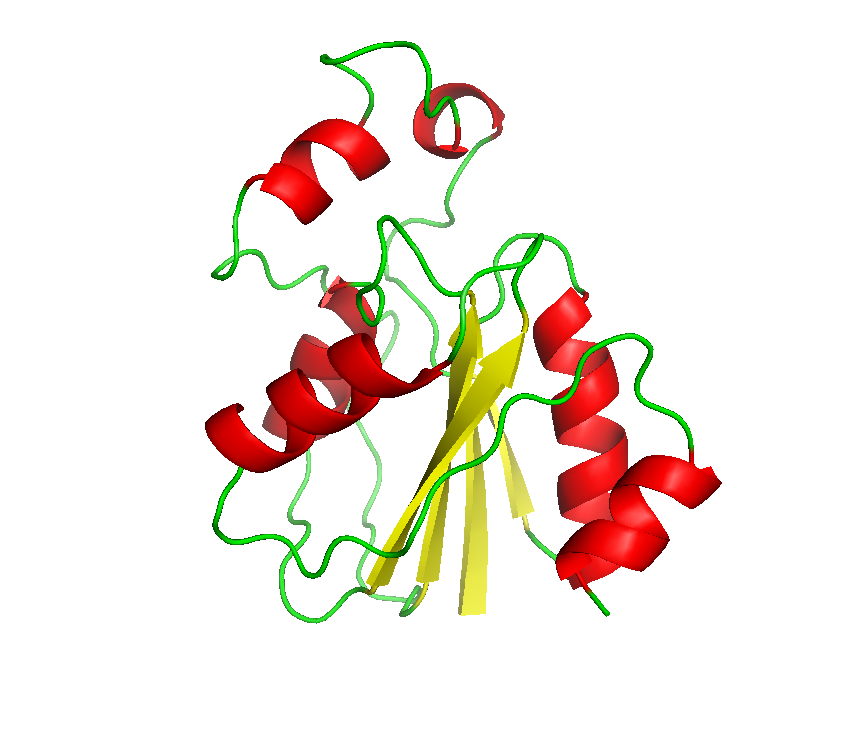
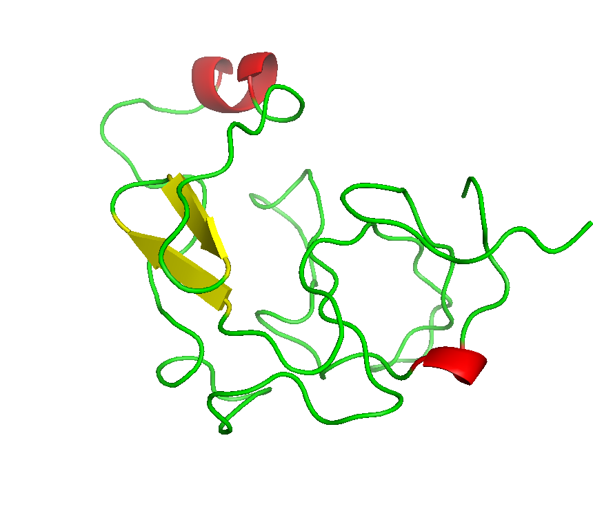
Final model from autoSHARP:
Files: 4J8P.pir 4J8P_truncate.mtz
% run_autoSHARP.sh \
  -seq 4J8P.pir -ha "Se" \
  -wvl 0.97858 peak -8.000 6.000  -mtz 4J8P_truncate.mtz \
  -id autoSHARP_SAD2 | tee autoSHARP_SAD2.lis
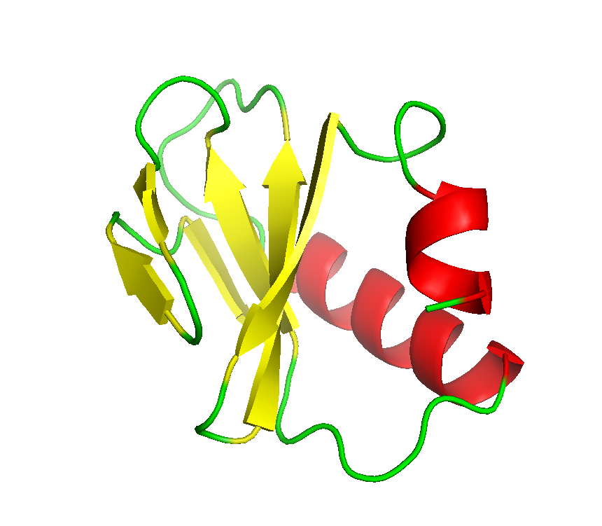
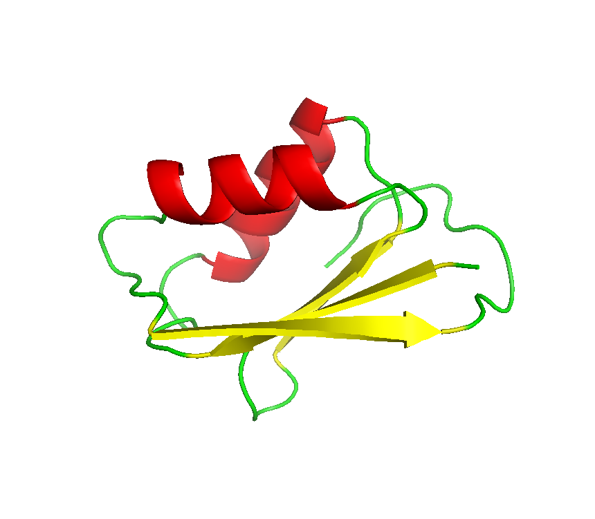
Final model from autoSHARP:
MAD
Files: 4JM1.pir 4JM1_truncate_0.97849.mtz 4JM1_truncate_0.97917.mtz
% run_autoSHARP.sh \
  -seq 4JM1.pir -ha "Se" \
  -wvl 0.97849 peak -4.660 4.060  -mtz 4JM1_truncate_0.97849.mtz \
  -wvl 0.97917 infl -7.690 2.050  -mtz 4JM1_truncate_0.97917.mtz \
  -id autoSHARP_MAD-2wvl | tee autoSHARP_MAD-2wvl.lis
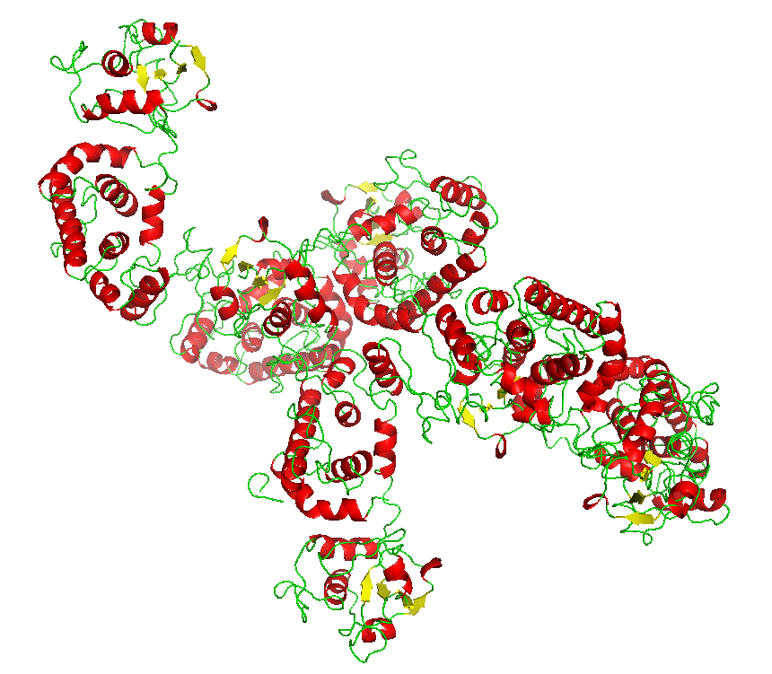
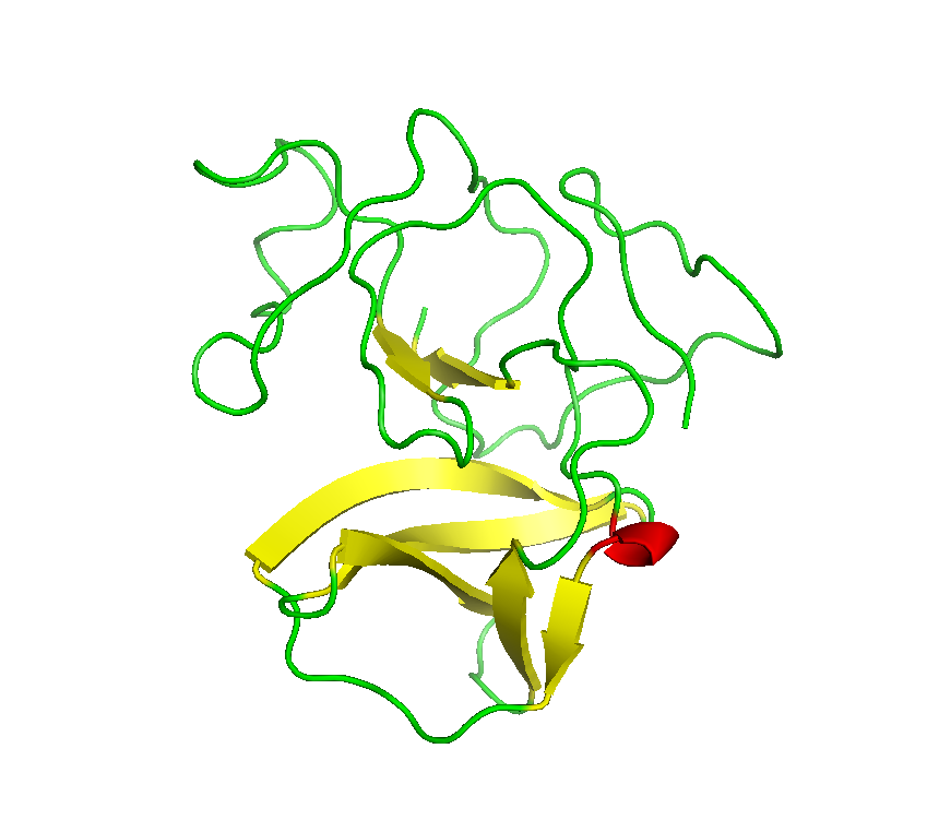
Final model from autoSHARP:
Files: 4IS3.pir 4IS3_truncate_0.91162.mtz 4IS3_truncate_0.97919.mtz 4IS3_truncate_0.97936.mtz
% run_autoSHARP.sh \
  -seq 4IS3.pir -ha "Se" \
  -wvl 0.97936 infl -11.400 3.710  -mtz 4IS3_truncate_0.97936.mtz \
  -wvl 0.91162 hrem  -1.700 3.300  -mtz 4IS3_truncate_0.91162.mtz \
  -wvl 0.97919 peak  -8.700 6.670  -mtz 4IS3_truncate_0.97919.mtz \
  -id autoSHARP_MAD-3wvl | tee autoSHARP_MAD-3wvl.lis
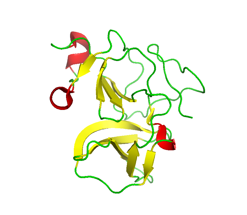
Final model from autoSHARP:
Files: 4ME8.pir 4ME8_truncate_0.97944.mtz 4ME8_truncate_0.91837.mtz 4ME8_truncate_0.97894.mtz
% run_autoSHARP.sh \
  -seq 4ME8.pir -ha "Se" \
  -wvl 0.97944 infl -8.600 2.660  -mtz 4ME8_truncate_0.97944.mtz \
  -wvl 0.91837 hrem -1.800 3.400  -mtz 4ME8_truncate_0.91837.mtz \
  -wvl 0.97894 peak -6.860 4.580  -mtz 4ME8_truncate_0.97894.mtz \
  -id autoSHARP_MAD2-3wvl | tee autoSHARP_MAD2-3wvl.lis
Final model from autoSHARP:
SIRAS
Files: 1GXT.pir 1GXT_nat.mtz 1GXT_hg.mtz
% run_autoSHARP.sh \
  -seq 1GXT.pir \
  -nat -mtz 1GXT_nat.mtz \
  -ha "Hg" -nsit 2 -wvl 0.99970 peak -16 10 -mtz 1GXT_hg.mtz \
  -id autoSHARP_SIRAS | tee autoSHARP_SIRAS.lis
Final model from autoSHARP:
MIRAS
Files: 3ZFT.pir 3ZFT_nat.mtz 3ZFQ_Hg.mtz 3ZFR_Ir.mtz
% run_autoSHARP.sh \
  -seq 3ZFT.pir -nat -mtz 3ZFT_nat.mtz \
  -ha "Hg" -nsit 1 -wvl 1.54179 -mtz 3ZFQ_Hg.mtz \
  -ha "Ir" -nsit 2 -wvl 1.54179 -mtz 3ZFR_Ir.mtz \
  -id autoSHARP_MIRAS | tee autoSHARP_MIRAS.lis
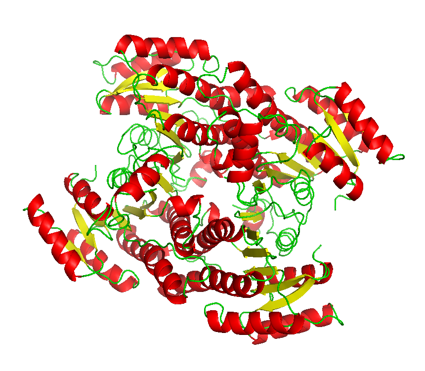
Final model from autoSHARP compared to deposited structure:
Including partial model
Files: 3GET.pir 3FFH_ala_MR.pdb 3GET.sca
% run_autoSHARP.sh \
  -seq 3GET.pir -ha "Se" \
  -pdb 3FFH_ala_MR.pdb \
  -wvl 0.9789 peak -8 4 -sca 3GET.sca \
  -id autoSHARP_SAD-MR | tee autoSHARP_SAD-MR.lis
This case has been chosen in such a way that (1) the experimental phasing signal is not too strong and needs "rescuing" by a partial model, and (2) that partial model itself is sufficiently poor that its phase information doesn't totally dominate over the experimental one. Therefore, the overall phase quality will be marginal and the results arrived at automatically by autoSHARP cannot be expected to be spectacular - indeed, it would be a bad example if they were.
Final model from autoSHARP compared to deposited structure: