Content:
- Introduction
- Data processing with autoPROC (about 5 minutes)
- Structure solution with SHARP/autoSHARP (about 15 minutes)
- Structure refinement with BUSTER (about 15 minutes)
Introduction
This is an attempt of giving an introduction to our main software components within a very short time. It only gives a taster, but should be enough to get you started. Much more introductory material is available for each program:
Because of the limited time available for this demo, sometimes non-default options will be used to speed things up. Those will be clearly indicated.
Whenever timings are given, they are for a i7-2720QM laptop with 8Gb of memory.
Data processing with autoPROC
Some examples and tutorials are given on the autoPROC wiki.
We're going to use the data for 1O22 from the JCSG. It is
- a 170 residue protein
- expressed with Se-MET (6 Met in sequence)
- data collected at the peak wavelength (0.9778 A)
- a fluorescence scan gave values of f'=-7 and f"=5.0
- detailed information available here
This peak dataset consists of 90 images (tm0875_8p44_1_E1_001.img to tm0875_8p44_1_E1_090.img). We can run this with some additional automation using the process command from a terminal/shell:
% cd /where/ever/images
% process -M automatic -d 01 | tee 01.lis
which should give us after about 3 minutes a processed dataset (using XDS, POINTLESS and SCALA/AIMLESS as part of autoPROC) with
                                            Overall  InnerShell  OuterShell
---------------------------------------------------------------------------
   Low resolution limit                      38.229      38.229       1.958
   High resolution limit                      1.951       8.544       1.951

   Rmerge                                     0.061       0.034       0.491
   Ranom                                      0.050       0.026       0.445
   Rmeas (within I+/I-)                       0.059       0.030       0.545
   Rmeas (all I+ & I-)                        0.066       0.038       0.555
   Rpim  (within I+/I-)                       0.031       0.016       0.307
   Rpim  (all I+ & I-)                        0.025       0.016       0.249
   Total number of observations               84852        1077         669
   Total number unique                        13110         207         151
   Mean(I)/sd(I)                               24.9        57.3         2.8
   Completeness                                97.4       100.0       100.0
   Multiplicity                                 6.5         5.2         4.4

   Anomalous completeness                      95.4        95.7        94.0
   Anomalous multiplicity                       3.6         3.6         2.4
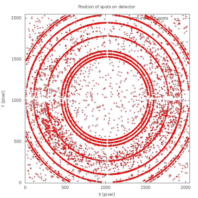
There are a few interesting warnings/notes from this data processing run. First we get
WARNING : the selected indexing solution uses less than 80%
          of initial spots - please check this carefully for
          ice-rings or minor lattices.

NOTE : automatically added 10 EXCLUDE_RESOLUTION_RANGE
       cards - based on automatic analysis (see
       01/xds_spots2res.log for details)
which is due to ice-rings - shown in image 01/SPOT.noHKL.png:
Structure solution with SHARP/autoSHARP
Please have a look at the examples and tutorials on the SHARP/autoSHARP wiki.
We can use the data just processed for solving the structure with autoSHARP (run through the Sushi http-interface). Apart from switching on the fast path
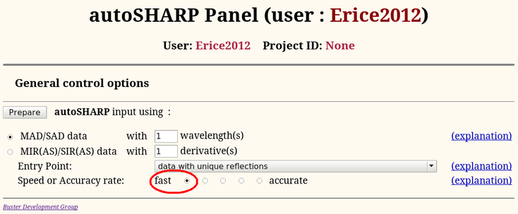 |
we're going to use all defaults:
- sequence file 1o22.pir
- searching for 6 Se atoms
- wavelength 0.9778 A
- f' and f" values of -7 and +5
- reflection file from autoPROC 1o22_peak.sca
After about 10 minutes we should have
- found the heavy atom sites (with SHELXC/D)
- refined these, calculated phases (with SHARP)
- density modified the experimental map (with SOLOMON)
- built an initial map (using ARP/wARP, REFMAC)
This model has 145 out of 170 residues buit with R/Rfree = 0.219/0.259 :
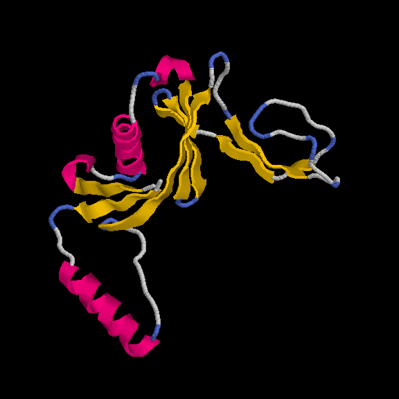 Remember, the deposited model contains 149 residues - so we are basically finishing with a complete model.
Structure refinement with BUSTER
Please make sure to have a BUSTER reference card handy. You should also check the various examples, tutorials and FAQs on the BUSTER wiki.
We can take the first (already very good) model and MTZ file - eden_flat_47.8pc_warpNtrace.pdb and eden_flat_47.8pc_warpNtrace.mtz - to run refinement with BUSTER on it. There are a few things we might want to remember at this stage:
- we need to change the built MET residues to become MSE (Se-MET) residues (you could use the jiffy met2mse.sh for that)
- the formfactor for Se needs to be adjusted by the known f' value ([-7])
First create a corrected PDB file with
% met2mse.sh eden_flat_47.8pc_warpNtrace.pdb
to give us eden_flat_47.8pc_warpNtrace_MSE.pdb:
Then let's first run a simple map-calculation with BUSTER ussing the refine command from a terminal/shell:
% refine -p eden_flat_47.8pc_warpNtrace_MSE.pdb \
         -m eden_flat_47.8pc_warpNtrace.mtz \
         FormfactorCorrection="Se:-7" \
         -M MapOnly -d BUSTER.01 | tee BUSTER.01.lis
which gives us R/Rfree = 0.225/0.261 (quite similar to the values from the ARP/wARP stage of autoSHARP).
A more complete initial refinement with BUSTER at this stage could be run with
% refine -p eden_flat_47.8pc_warpNtrace_MSE.pdb \
         -m eden_flat_47.8pc_warpNtrace.mtz \
         FormfactorCorrection="Se:-7" \
         -M WaterUpdatePkmaps -M TLSbasic \
         -d BUSTER.02 | tee BUSTER.02.lis
which results in R/Rfree = 0.199/0.244 after about 8 minutes (remember that read BUSTER refine jobs runs several so-called BIG cycles where eg. bulk solvent mask and solvent structure are updated):
How does the model geometry improve? Looking at some MolProbity scores:
before:
 ___________________________________________________________________________
|        |Clashscore, all atoms:   |23.08 |25th percentile* (N=1784, all    |
|All-Atom|_________________________|______|resolutions)_____________________|
|Contacts|Clashscore is the number of serious steric overlaps (> 0.4 AA) per|
|________|1000_atoms._______________________________________________________|
|        |Poor_rotamers____________|5.93%_|Goal:_<1%________________________|
|        |Ramachandran_outliers____|0.00%_|Goal:_<0.2%______________________|
|        |Ramachandran_favored_____|98.62%|Goal:_>98%_______________________|
|Protein |Cb_deviations_>0.25AA____|1_____|Goal:_0__________________________|
|Geometry|MolProbity score^        |2.44  |50th percentile* (N=27675, 0AA - |
|        |_________________________|______|99AA)____________________________|
|        |Residues_with_bad_bonds:_|0.00%_|Goal:_0%_________________________|
|________|Residues_with_bad_angles:|0.00%_|Goal:_<0.1%______________________|
after BUSTER refinement:
 ____________________________________________________________________________
|        |Clashscore, all atoms:   |5.36  |96th percentile* (N=821, 1.95AA +/|
|All-Atom|_________________________|______|-_0.25AA)_________________________|
|Contacts|Clashscore is the number of serious steric overlaps (> 0.4 AA) per |
|________|1000_atoms.________________________________________________________|
|        |Poor_rotamers____________|4.44%_|Goal:_<1%_________________________|
|        |Ramachandran_outliers____|0.00%_|Goal:_<0.2%_______________________|
|        |Ramachandran_favored_____|99.31%|Goal:_>98%________________________|
|Protein |Cb_deviations_>0.25AA____|1_____|Goal:_0___________________________|
|Geometry|MolProbity score^        |1.78  |85th percentile* (N=13349, 1.95AA |
|        |_________________________|______|+/-_0.25AA)_______________________|
|        |Residues_with_bad_bonds:_|0.00%_|Goal:_0%__________________________|
|________|Residues_with_bad_angles:|0.00%_|Goal:_<0.1%_______________________|
We can now checking the structure against the density (plus geomeric problems) using
% visualise-geometry-coot BUSTER.02
After improving the model interactively, additional refinement jobs could be run either directly through the Coot interface or again on the command-line.
Remember, please also read about grade (our geometric restraints generator) and the detailed examples.