Content:
What was the reason to pick this structure? It was one of the only 2 PDB entries with diffraction data deposited (thanks to the authors!) - so we might as well pick this one to also show how to (re-)process the raw diffraction images.
We can fetch the original, deposited data using
fetch_PDB 5VZRwhich will give use files
5VZR/5vzr.pdb
5VZR/5vzr.mtz
and various other diagnostics. All subsequent commands are run within the 5VZR subdirectory created by this command.
Note: all maps are shown at rms=1.0 (2mFo-DFc) and rms=3.5 (mFo-Dfc) levels unless stated otherwise.
There are multiple ways of looking at electron density maps for a given PDB entry. The easiest is to use the tools from one of the wwPDB sites, e.g. https://www.rcsb.org/3d-view/5VZR?preset=electronDensityMaps. But if you are more familiar with using Coot, you should be able to load both model and electron density (2mFo-DFc) and difference (mFo-Dfc) maps from within the Coot interface. You could also go directly to PDB-REDO and look at the available models and maps.
Often, PDB entries will contain the map-coefficients of the maps as originally seen by the depositor/author (items _refln.pdbx_FWT, _refln.pdbx_PHWT, _refln.pdbx_DELFWT and _refln.pdbx_DELPHWT in the structure factor mmCIF file). 1
Here we are going to use the so-called "MapOnly" mode in BUSTER, namely running
  refine -M MapOnly -p 5vzr.pdb -m 5vzr.mtz -d MapOnly | tee MapOnly.lis
  cd MapOnly
  coot --pdb refine.pdb --auto refine.mtz
So we are not doing any refinement of the deposited model (apart from the overall scaling model) and compute the different types of maps.
What can we see (in order of largest difference map peaks)? Some examples showing a few possible, small corrections:
| Location | Maps | Remarks |
| A223 | 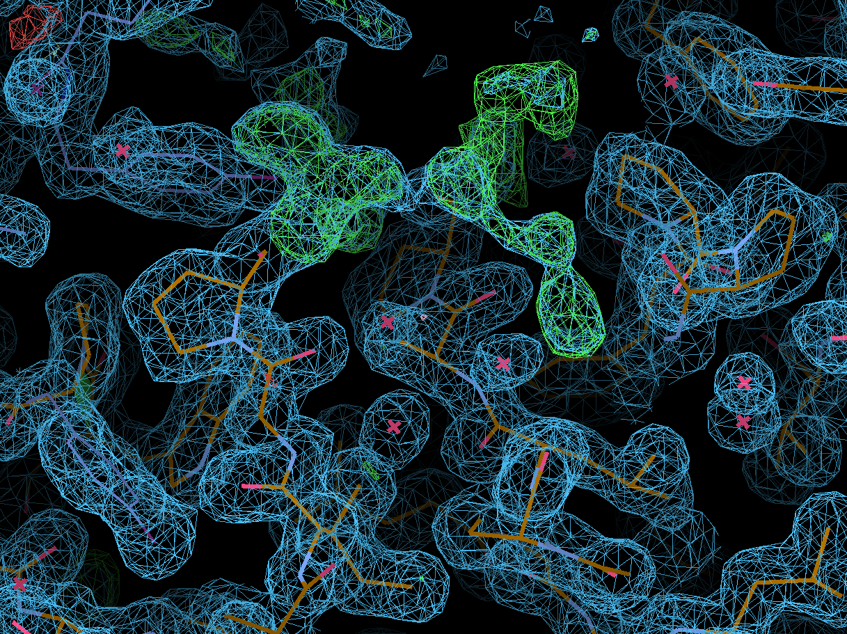 |
some density for additional residues (A224-A235 not yet modelled) |
| H61, H65 | 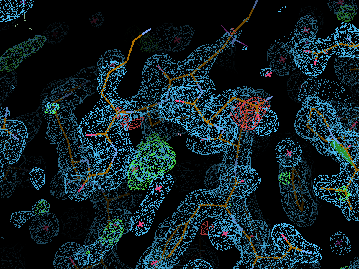 |
maybe alternate loop conformation and signs of radiation damage |
| H206 | 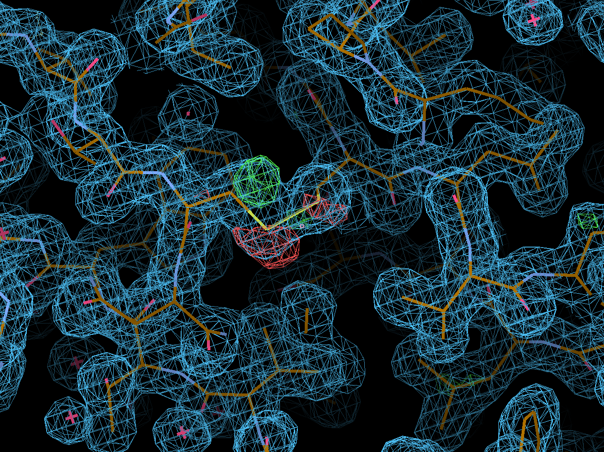 |
broken disulfide bond due to radiation damage |
| L188 | 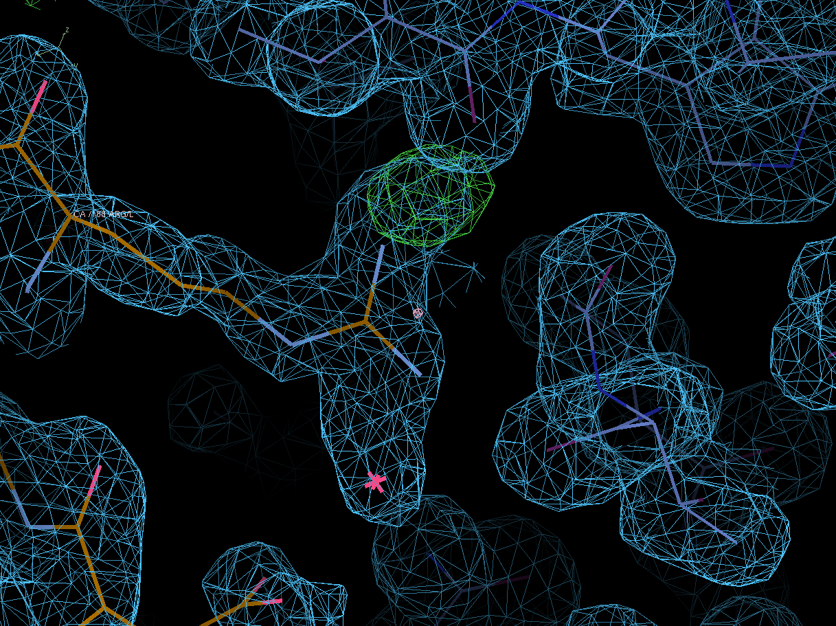 |
different rotamer with additional water? |
| H80 | 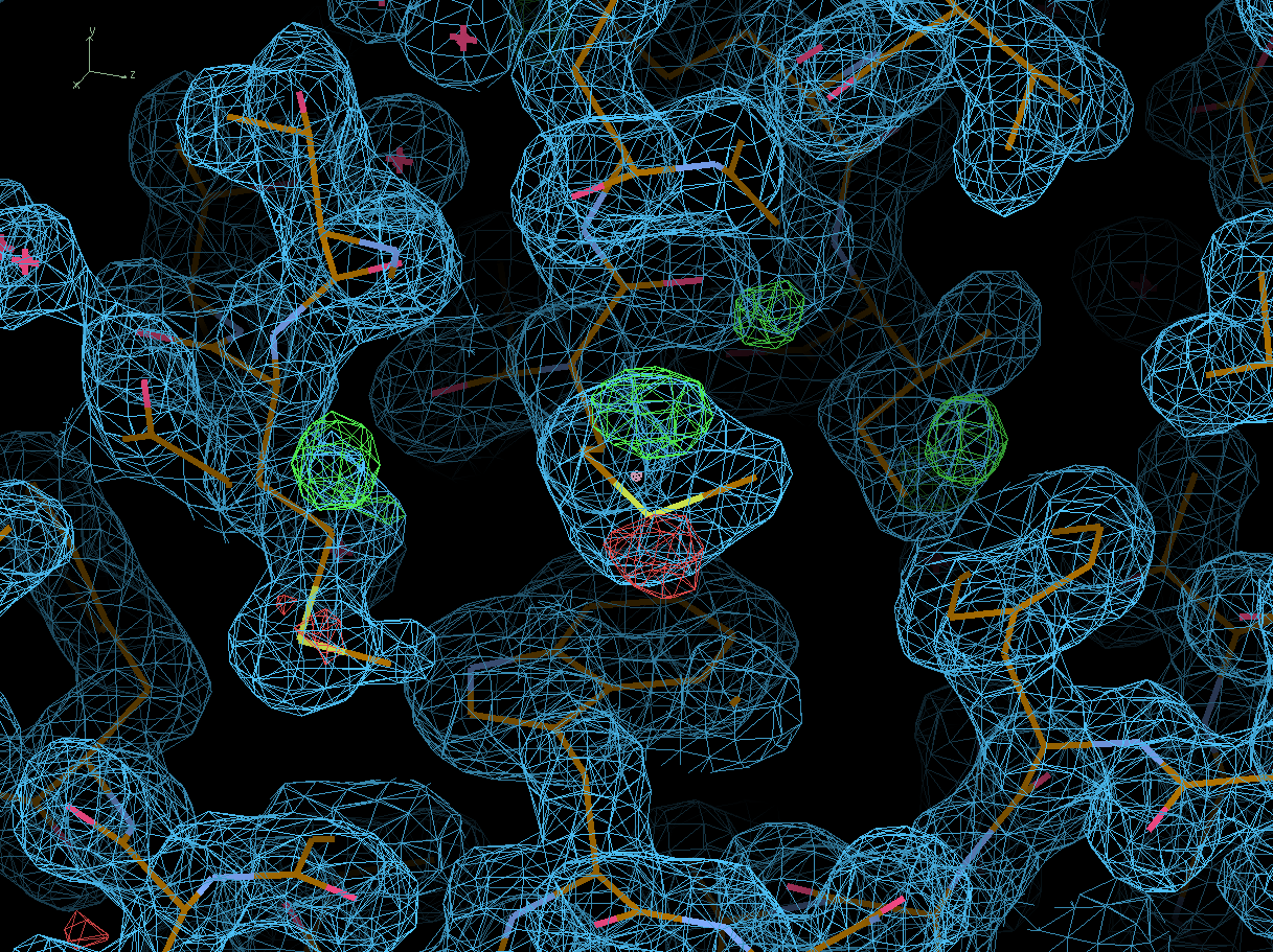 |
different/alternate rotamers |
| B11 | 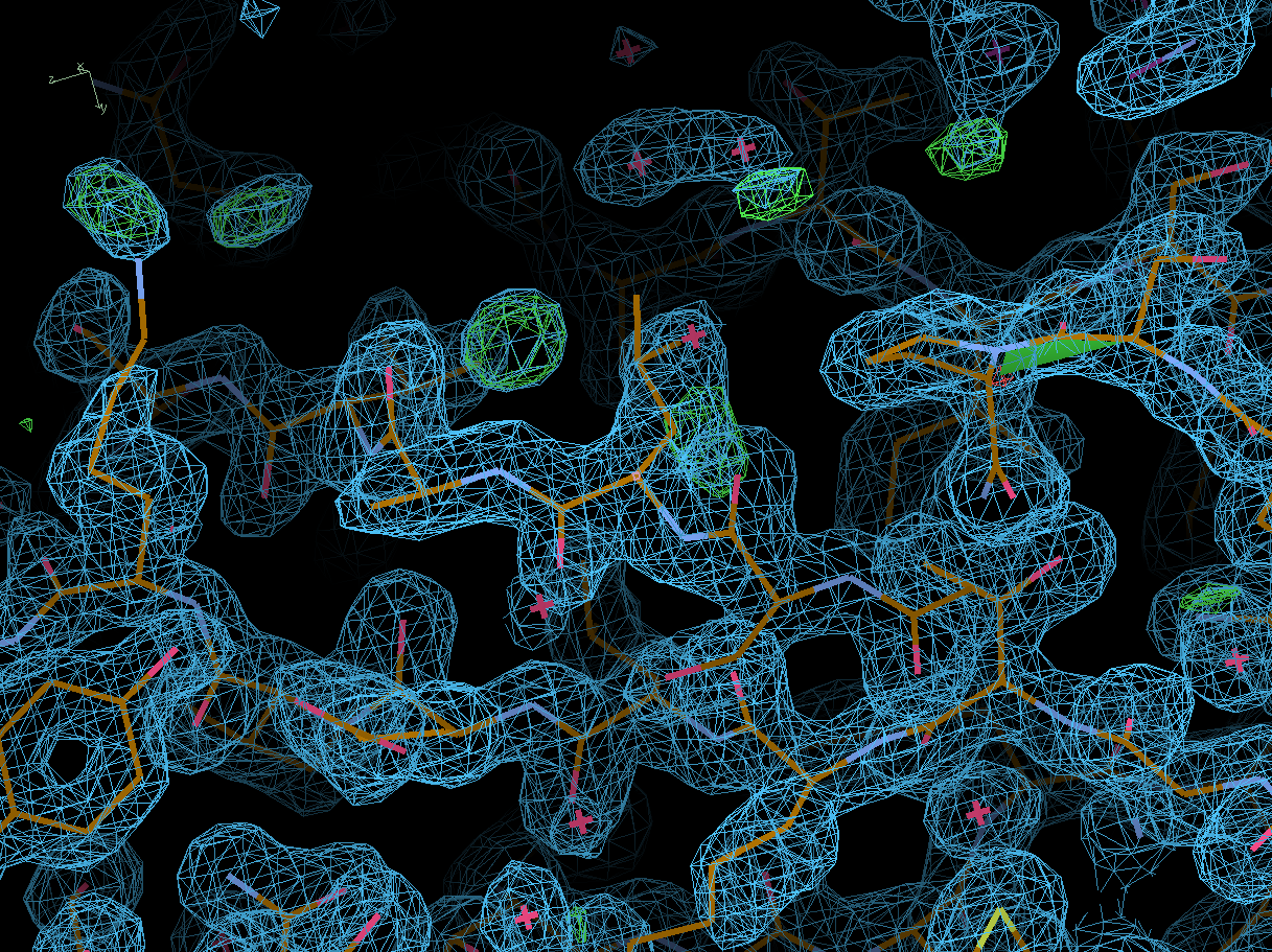 |
additional water |
| L194 | 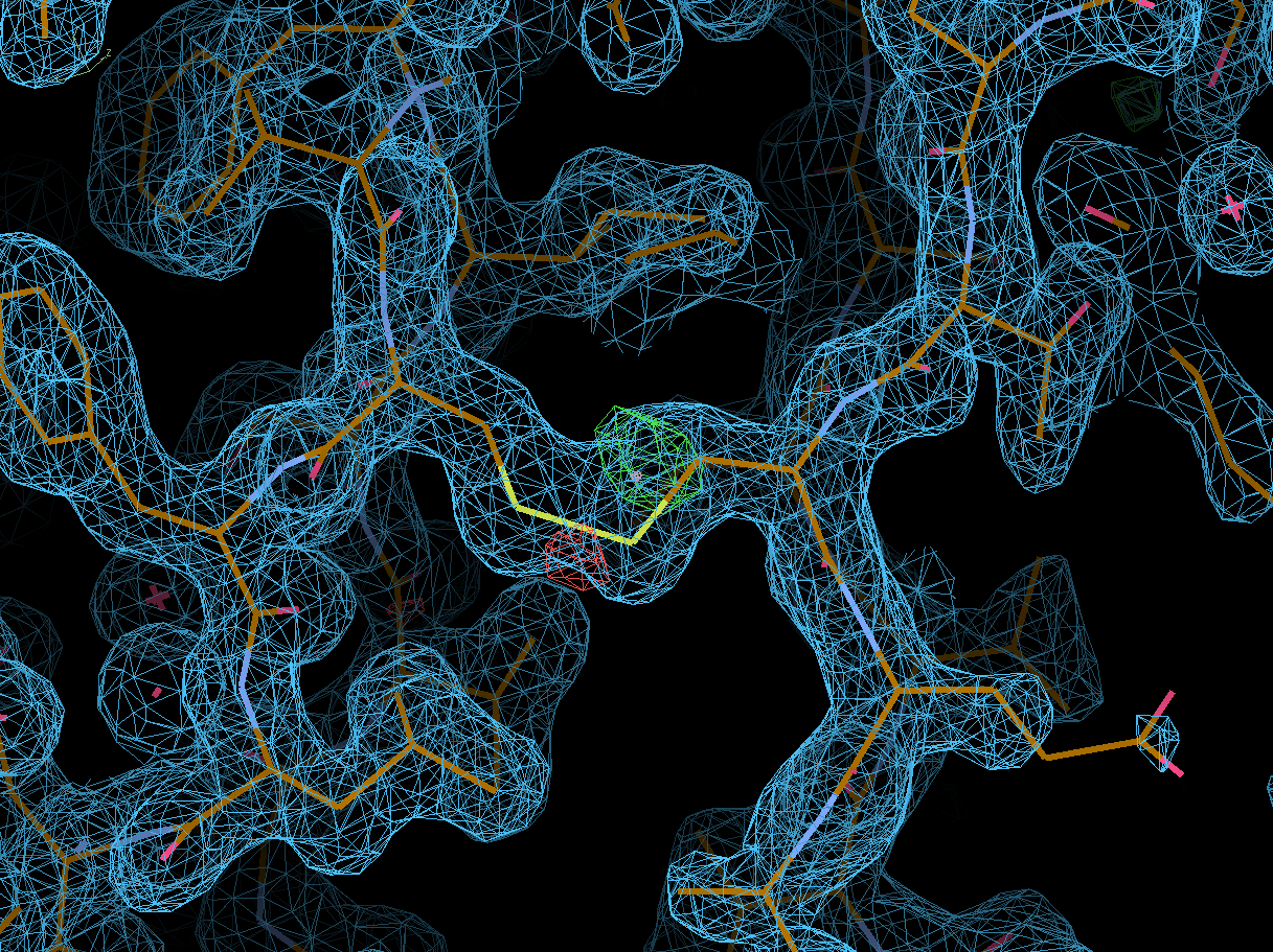 |
broken disulfide bond due to radiation damage |
| H43 | 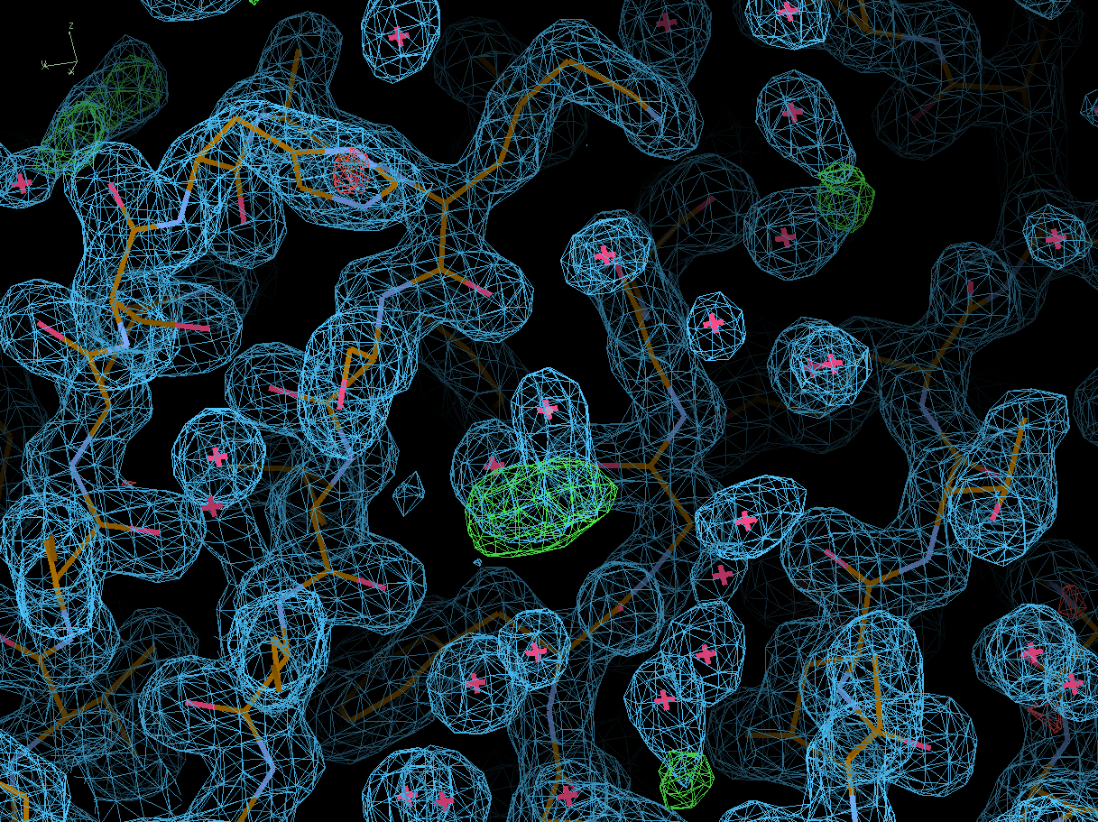 |
glycerol (GOL) molecule? |
| L103 | 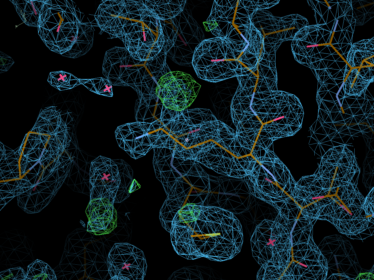 |
alternate conformation |
| Location | Maps | Remarks |
| A223 | 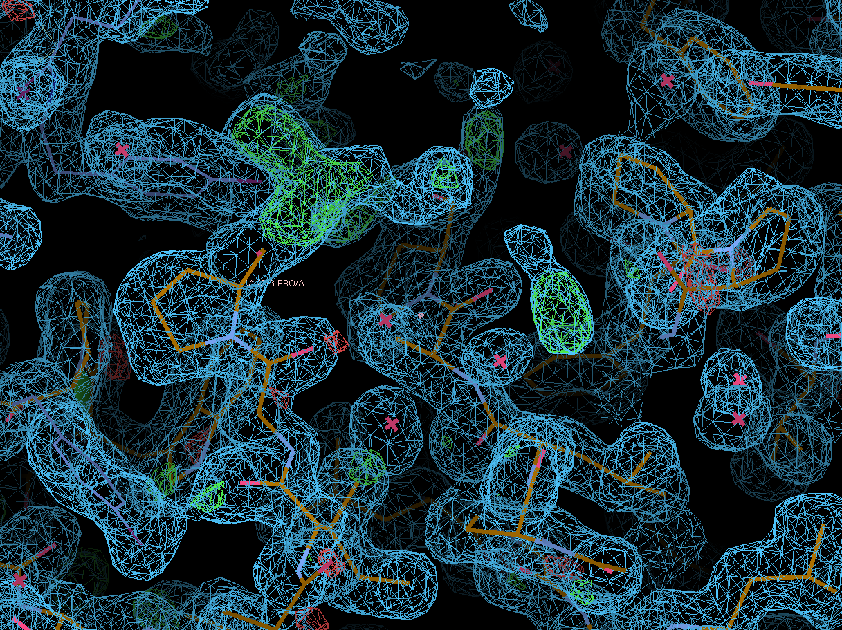 |
some density for additional residues (A224-A235 not yet modelled) |
| H61, H65 | 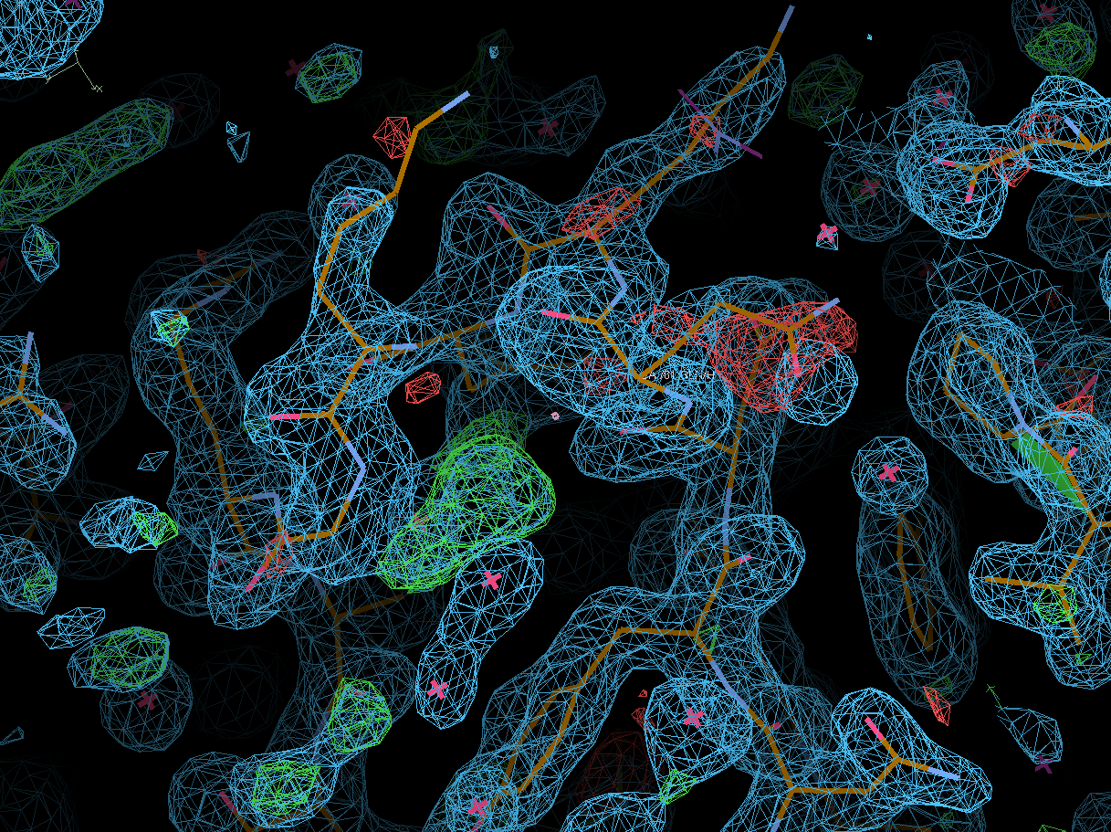 |
maybe alternate loop conformation and signs of radiation damage |
| H206 | 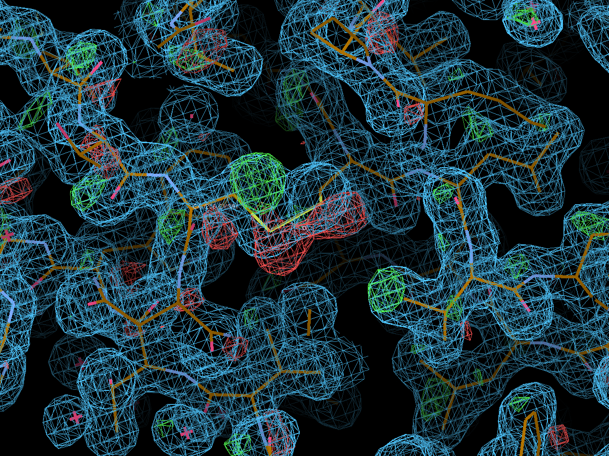 |
broken disulfide bond due to radiation damage |
| L188 | 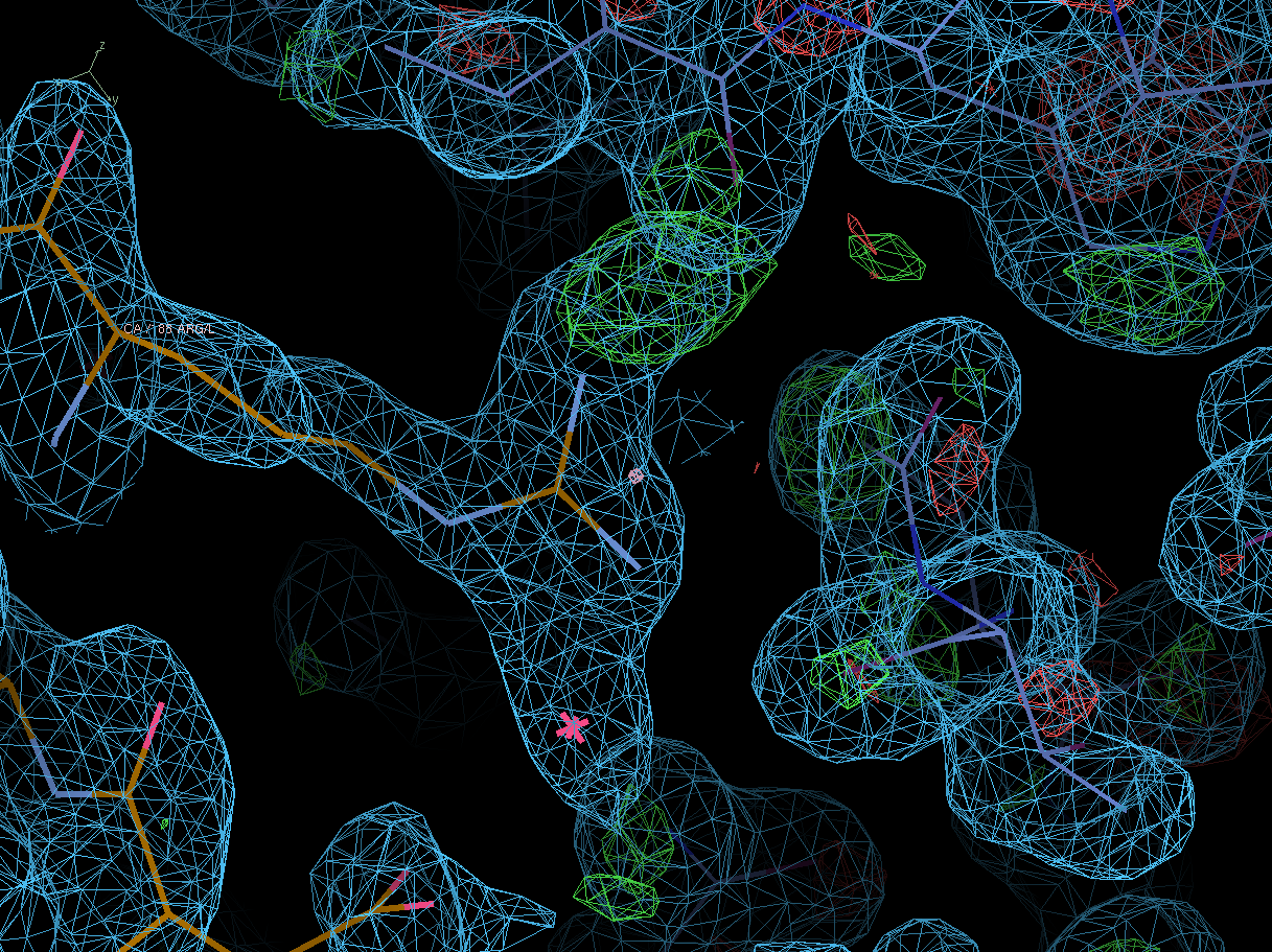 |
different rotamer with additional water? |
| H80 |  |
different/alternate rotamers |
| B11 | 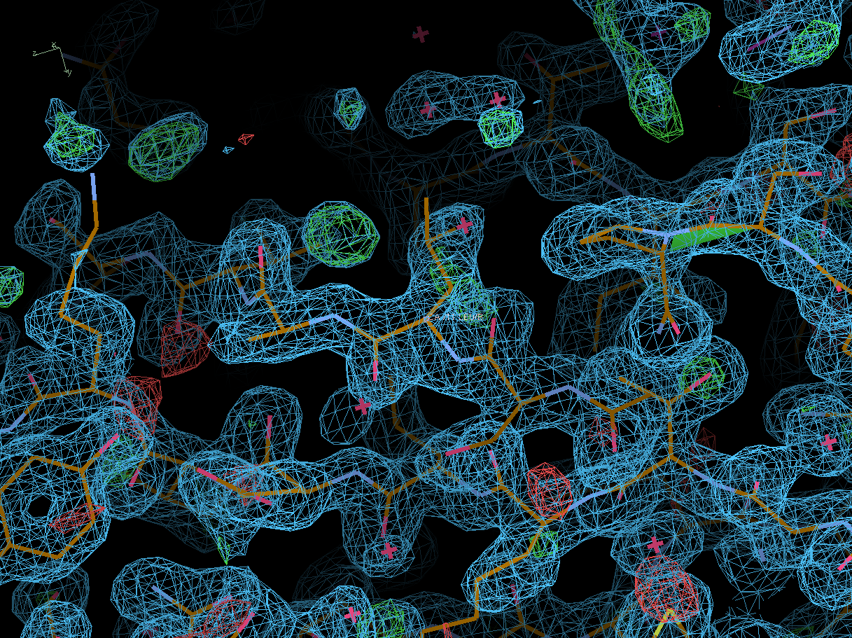 |
additional water |
| L194 | 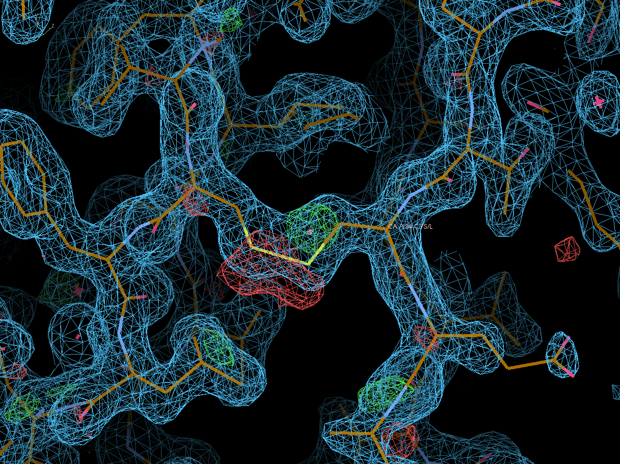 |
broken disulfide bond due to radiation damage |
| H43 | 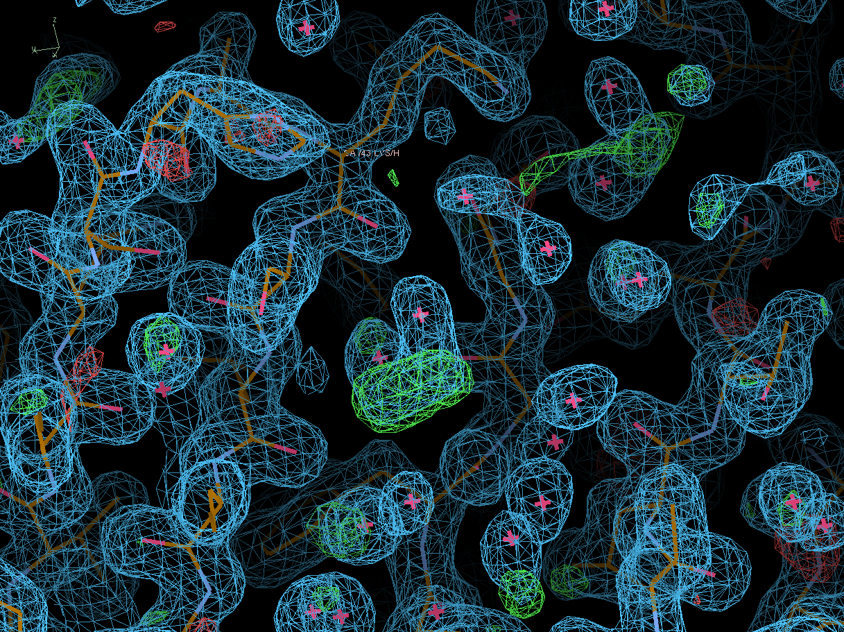 |
glycerol (GOL) molecule? |
| L103 | 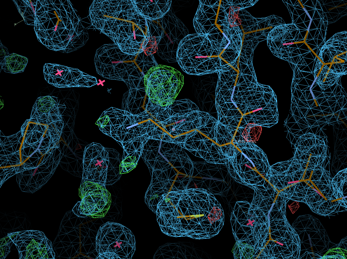 |
alternate conformation |
| Location | Maps | Remarks |
| A223 | 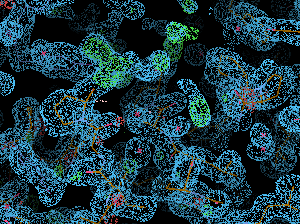 |
some density for additional residues (A224-A235 not yet modelled) |
| H61, H65 | 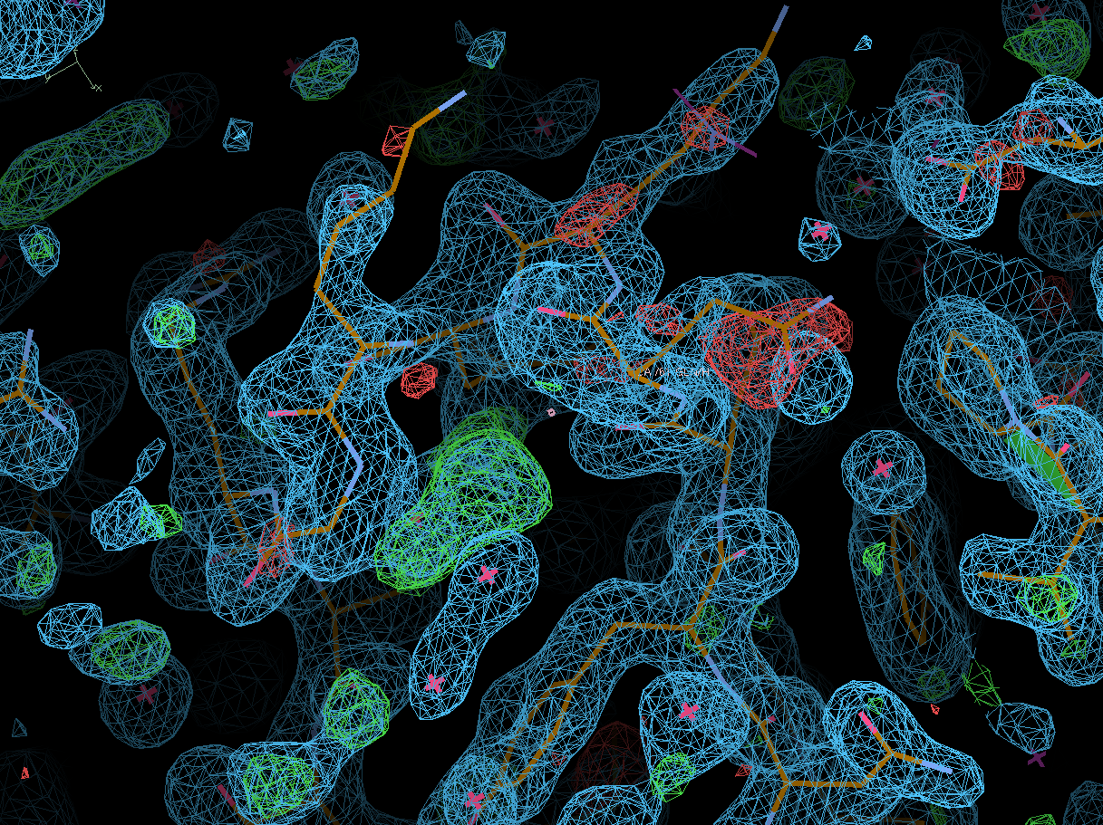 |
maybe alternate loop conformation and signs of radiation damage |
| H206 |  |
broken disulfide bond due to radiation damage |
| L188 | 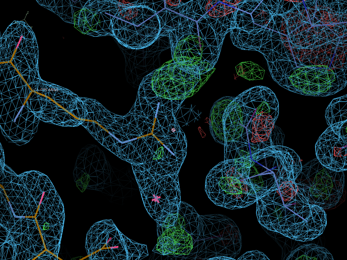 |
different rotamer with additional water? |
| H80 | 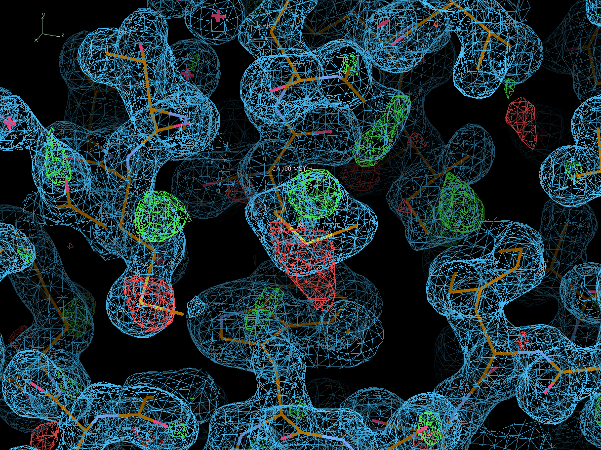 |
different/alternate rotamers |
| B11 | 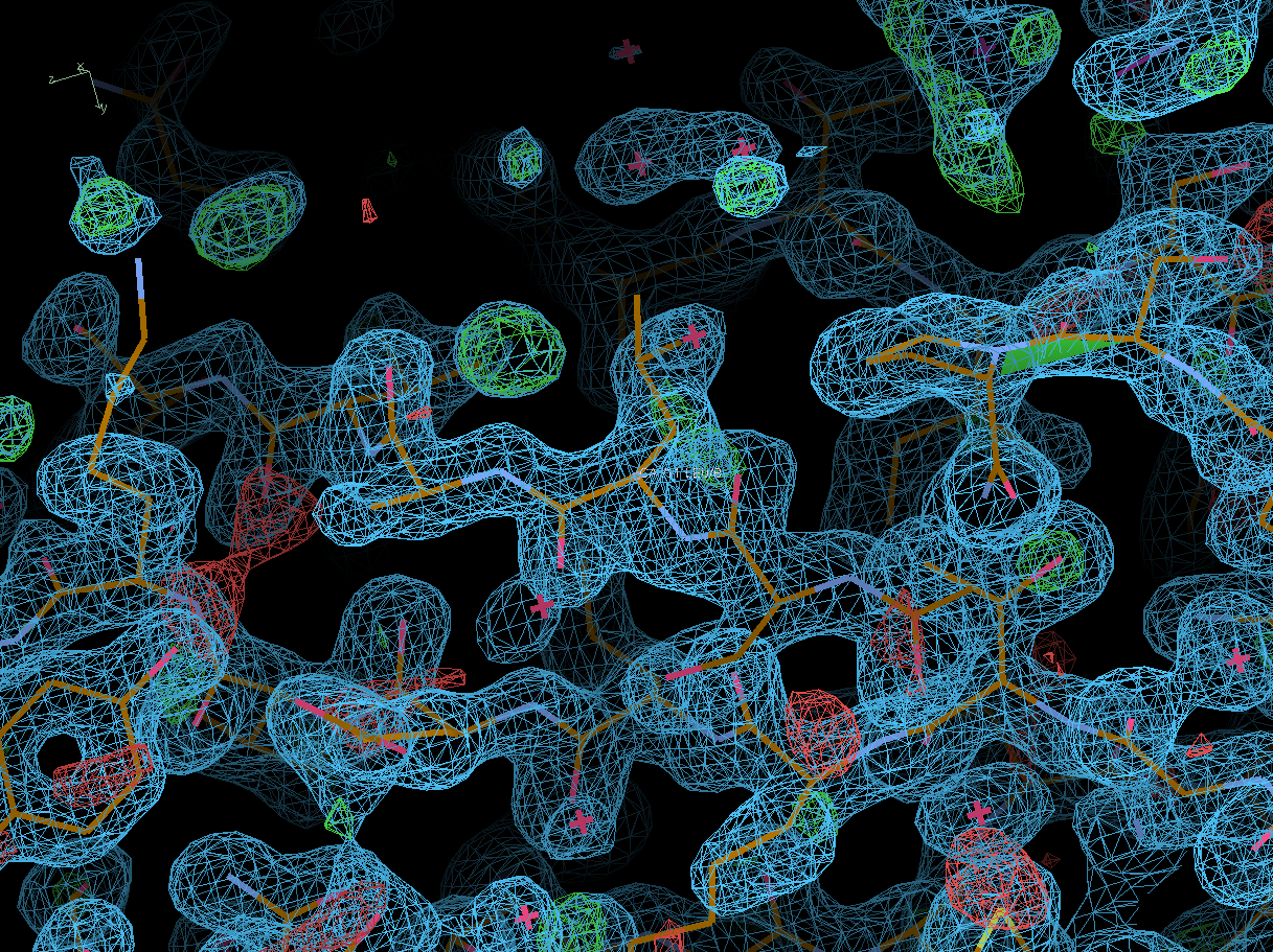 |
additional water |
| L194 |  |
broken disulfide bond due to radiation damage |
| H43 | 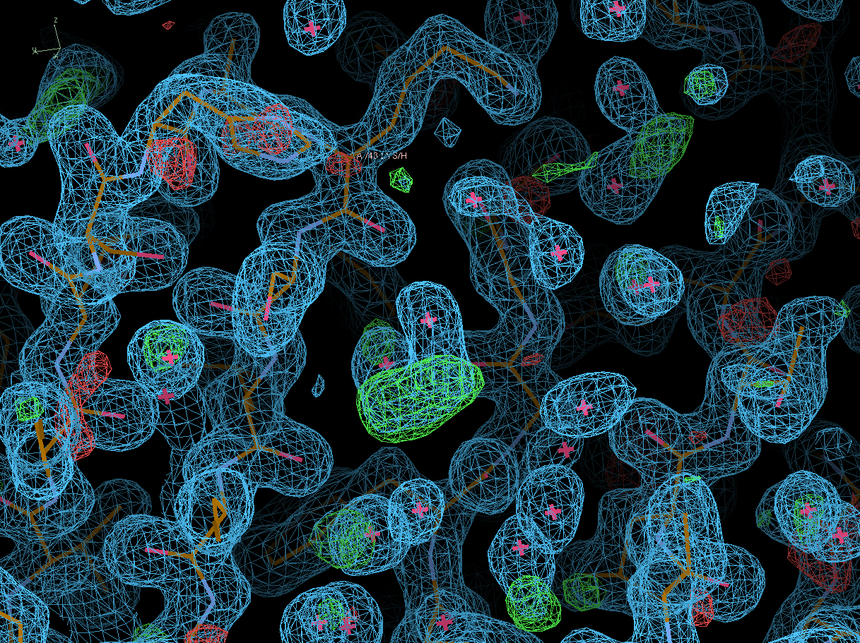 |
glycerol (GOL) molecule? |
| L103 | 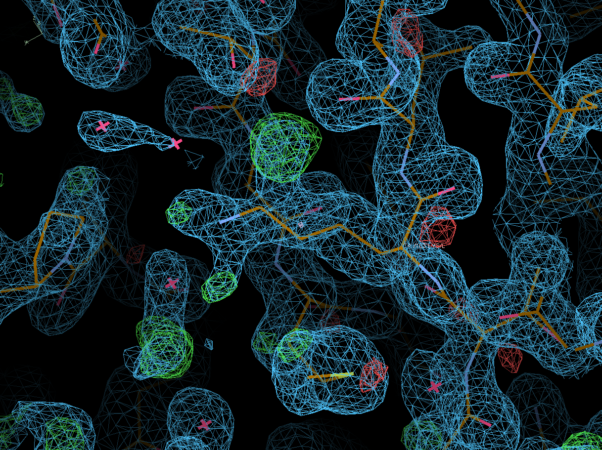 |
alternate conformation |
When there is enough multiplicity/redundancy in the data, autoPROC can merge distinct parts of the dataset into so-called "early" and "late" datasets. When such a reflection file (truncate-unique.mtz from autoPROC) is given to BUSTER it will create F(early)-F(late) difference Fourier maps that should show positive peaks where there was something at the beginning of data collection (atoms, electrons) and negative peaks where something appeared towards the end of data collection. So they are easy visualisations of potential radiation damage effects.
We also get a list of the highest positive peaks close to existing atoms, which would be those atoms/residues whihc are most likely damaged. Looking at those peaks (above 4.5 rms) here
Peak         Closest atom in aP_iso2.MapOnly/refine.pdb
[rms]                                             Distance (<= 1.0 )
------------------------------------------------------------------------
 10.10  <=>   SG  CYS B 194  (  1.00 31.27)  :       0.27
  7.78  <=>   SG  CYS L  88  (  1.00 18.68)  :       0.18
  7.65  <=>   SD  MET B  33  (  1.00 26.31)  :       0.36
  7.56  <=>   SG  CYS B  88  (  1.00 19.91)  :       0.48
  7.53  <=>   SG  CYS B  23  (  1.00 23.85)  :       0.38
  7.26  <=>   SG  CYS L  23  (  1.00 24.13)  :       0.32
  7.04  <=>   SD  MET L  33  (  1.00 26.26)  :       0.40
  6.76  <=>   SG  CYS B 134  (  1.00 21.97)  :       0.51
  6.49  <=>   SG  CYS L 194  (  1.00 40.76)  :       0.25
  6.05  <=>   SG  CYS H  22  (  1.00 17.90)  :       0.50
  5.93  <=>   SG  CYS A  22  (  1.00 20.65)  :       0.49
  5.77  <=>   SG  CYS A 206  (  1.00 24.34)  :       0.24
  5.68  <=>   SG  CYS A 140  (  1.00 22.55)  :       0.46
  5.64  <=>   SG  CYS H  92  (  1.00 15.67)  :       0.38
  5.32  <=>   SG  CYS A  92  (  1.00 17.29)  :       0.57
  5.24  <=>   SG  CYS H 140  (  1.00 22.66)  :       0.44
  5.21  <=>   O   HOH H 312  (  1.00 20.89)  :       0.56
  5.20  <=>   O   HOH H 365  (  1.00 23.87)  :       0.49
  5.19  <=>   CD  GLU L 123  (  1.00 47.18)  :       0.51
  5.17  <=>   O   ASP L 165  (  1.00 21.03)  :       0.70
  5.10  <=>   O   HOH H 426  (  1.00 30.93)  :       0.57
  4.98  <=>   OD2 ASP H  72  (  1.00 26.72)  :       0.65
  4.97  <=>   OD1 ASN H 207  (  1.00 20.02)  :       0.76
  4.93  <=>   OD1 ASP A 100C (  1.00 22.25)  :       0.68
  4.92  <=>   OE2 GLU L  27  (  1.00 50.86)  :       0.52
  4.85  <=>   OD2 ASP A 218  (  1.00 34.32)  :       0.49
  4.76  <=>   CG  ASP B  70  (  1.00 21.87)  :       0.76
  4.70  <=>   O   HOH B 393  (  1.00 19.92)  :       0.47
  4.69  <=>   O   HOH H 344  (  1.00 28.64)  :       0.62
  4.69  <=>   O   VAL H 217  (  1.00 15.41)  :       0.65
  4.69  <=>   CG2 THR H 205  (  1.00 15.67)  :       0.58
  4.68  <=>   CE BMET A  80  (  0.55 18.23)  :       0.52
  4.68  <=>   OG1 THR H 154  (  1.00 20.07)  :       0.66
  4.67  <=>   OD1 ASN L 137  (  1.00 18.09)  :       0.20
  4.67  <=>   SD  MET H 100E (  1.00 22.30)  :       0.61
  4.63  <=>   O   HOH A 453  (  1.00 40.93)  :       0.91
  4.62  <=>   OG  SER A 120  (  1.00 21.87)  :       0.84
  4.62  <=>   OD1 ASP L   1  (  1.00 33.52)  :       0.48
  4.62  <=>   OE1 GLU H 148  (  1.00 26.11)  :       0.72
  4.58  <=>   SG  CYS L 134  (  1.00 26.62)  :       0.77
  4.58  <=>   CG  ASP L 170  (  1.00 29.17)  :       0.61
  4.56  <=>   OD2 ASP L  27C (  1.00 30.67)  :       0.71
  4.53  <=>   OD1 ASP A 181  (  1.00 39.08)  :       0.32
  4.52  <=>   OD1 ASP A 218  (  1.00 28.37)  :       0.64
shows all the usual suspects: sulfurs CYS/MET residues mainly, but also some close to GLU/ASP carboxylates.
Looking at those maps in Coot (take columns F_early-late and PHI_early-late in the refine.mtz output file to create a difference map):
| B194 | 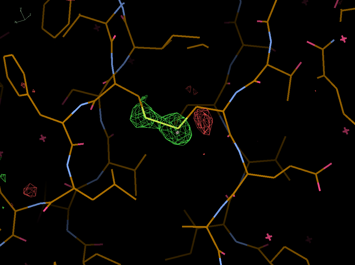 |
| B88 | 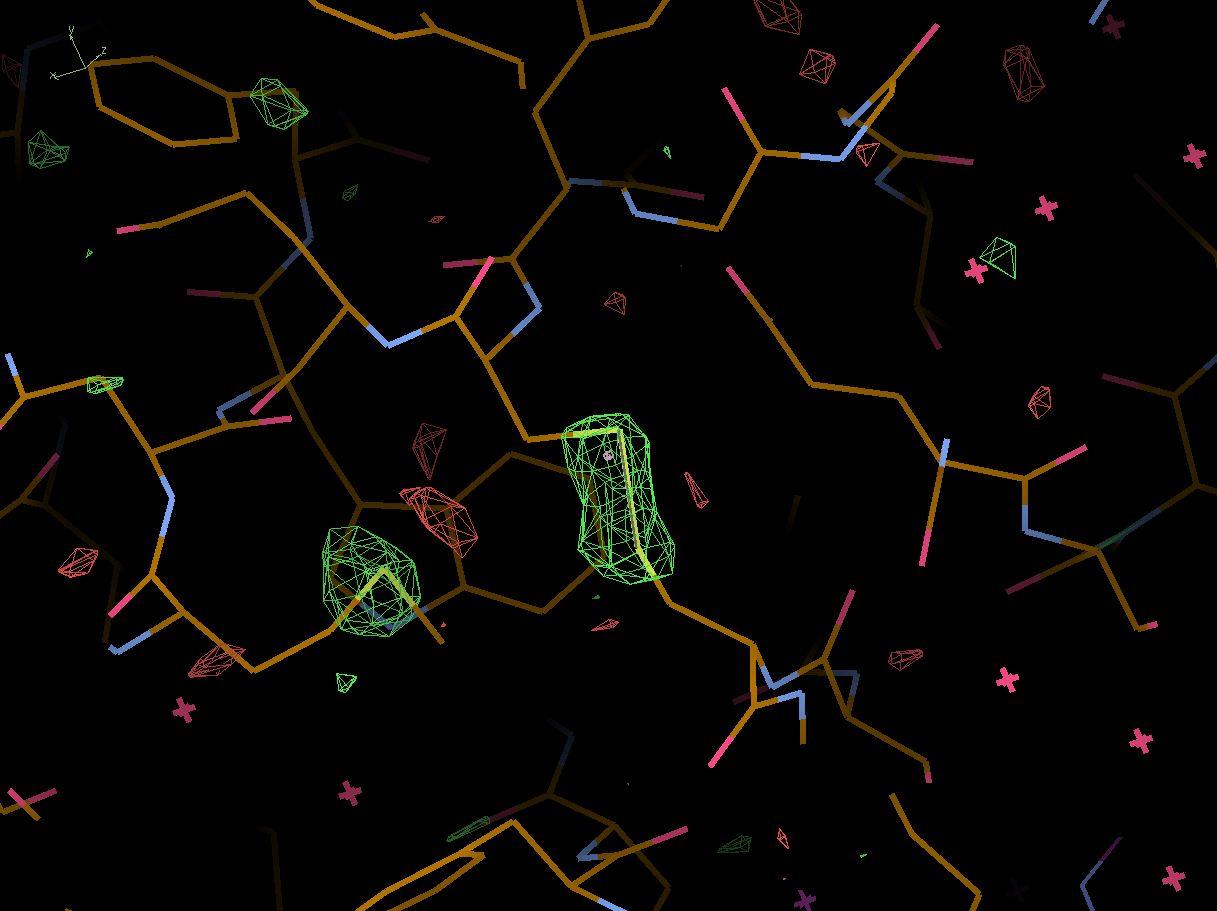 |
| L88 | 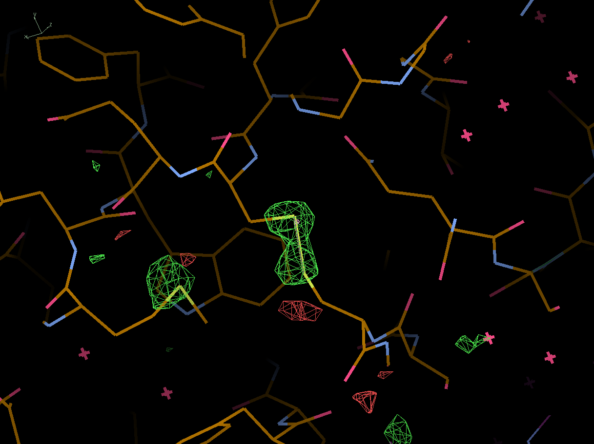 |
| B23 | 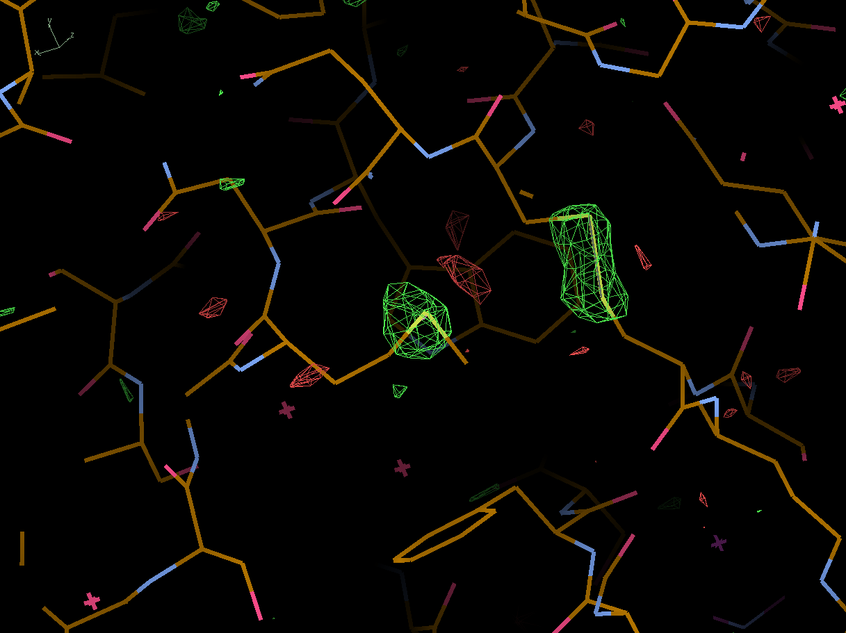 |
| L23 | 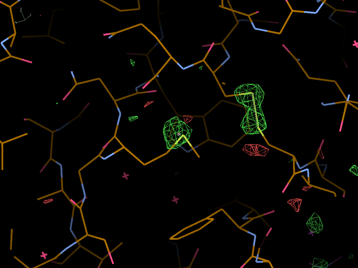 |
| A10 | 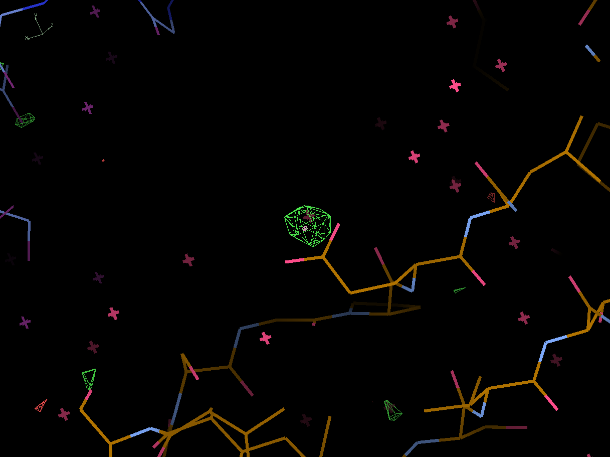 |
We are starting by using the anisotropic (STARANISO) analysed data from autoPROC, because: