Content 1 :
Revisiting existing datasets and structures always carries the risk of being seen as picky or a know-it all: this is never the intention here or in general. Datasets and models are always a result of their time and the circumstances: instruments improve, our knowledge how to use them increases, practices change, software gets better, time-pressure can be different and people have different backgrounds in general.
The idea here is to show on a few examples how we would be approaching the idea of revisiting existing datasets ... there are other ways of doing this and some will certainly be better or more appropriate than what we do here. But maybe these notes give you some ideas and pointers nevertheless.
The most important initial step is to collect all information about a particular dataset:
As of 20th March 2020, this is the newest (14th Nov 2019) pixel-array detector collected datasets for which raw images are deposited and recorded via their DOI at RCSB.
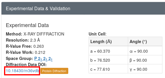
Looking at the RCSB page for this entry, we can see near the bottom left (in the "Experimental Data & Validation" section) a link to the proteindiffraction.org3 download page 4 :
 |
The download consists of a 6.4Gb tarball that we need to unpack somewhere, e.g.
  mkdir 6VDB
  cd 6VDB
  wget https://data.proteindiffraction.org/sgc/SETD2_HR606_6vdb.tar.bz2
  tar -xvf SETD2_HR606_6vdb.tar.bz2
This will give us a directory SETD2_HR606_6vdb/data with two datasets: a series of mini-cbf files for the Eiger dataset and a second dataset from a Rigaku Saturn A200 CCD detector. Since we are only interested in the Eiger dataset, we will simplify this via
  mkdir Images
  cd Images
  ln -s ../SETD2_HR606_6vdb/data/*.cbf .
  cd ../
We now have all relevant image files in the Images subdirectory (via symbolic links).
Using autoPROC5 we can just run
process -I Images -d 00 | tee 00.lisWhat do these arguments mean:
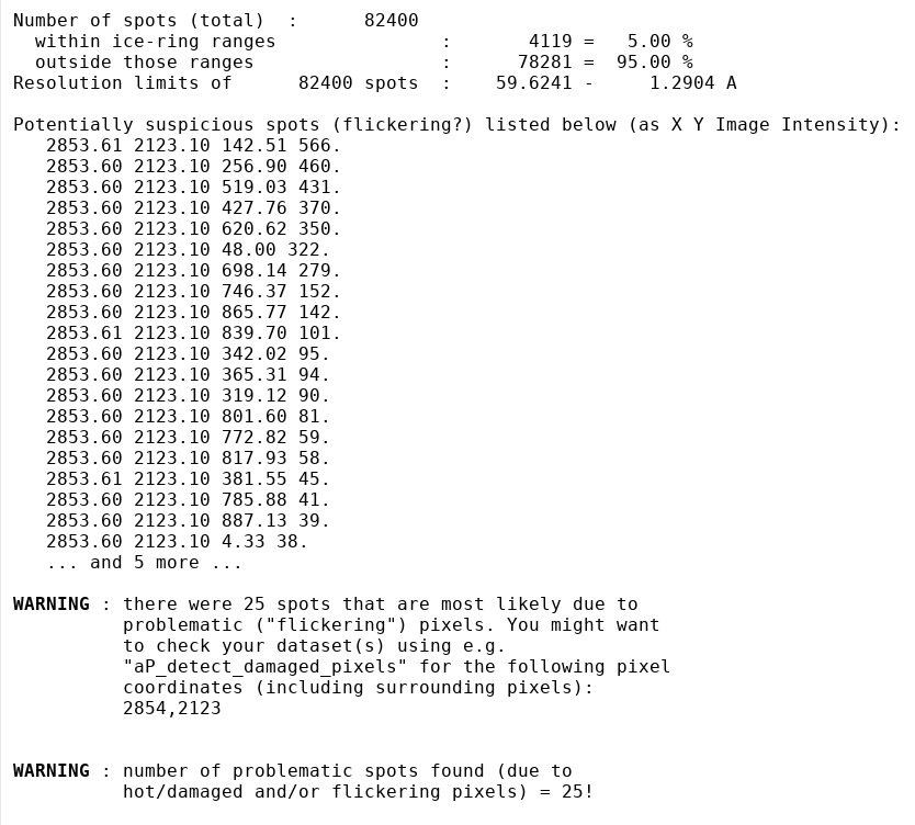
What potentially interesting messages do we get from this run? Typically, we would firs tlook at any WARNING messages - the first relevant one:
in standard output (detailed):
 |
in summary.html:
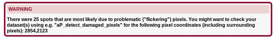 |
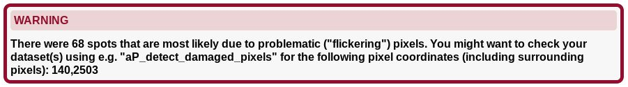
As you can see, there is a surprisingly large number of spots found by XDS/COLSPOT with the same (X,Y) coordinates. This looks suspiciously like a flickering pixel and we are excluding those spots from indexing. They would most likely not have a detrimental effect on the very robust indexing in IDXREF, but since it is done automatically it might help some much more borderline datasets ... better safe than sorry.
The next warning occurs during indexing itself:
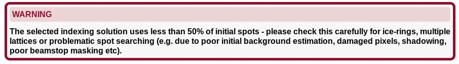 |
This is unexpected, since we would assume any spot found in the dataset comes from diffraction of a single crystal hit by the beam. A bit further up we see
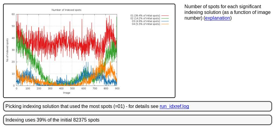 |
We seem to be dealing with a slightly messy diffraction pattern it seems (with various possible reasons for this). The important bit is that we picked the most prominent lattice during indexing - which might not have been possible if taking only very few images from the start of the dataset where two collections of spots seem to be nearly equally prominent.
We can see the relation between those (most prominent) indexing solutions
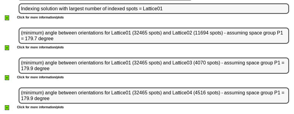 |
Remember that this indexing is all done in P1 and the relative angles between different orientation matrices (for each indexing solution) might be symmetry-related - so an angle of 179.7 might actually be just 0.3 degree (which then could point to slightly split spots or such). The different indexing solutions are visualised through prediction images (expand the green "+" button). Here are some closeups of those predictions:
| Lattice 01 | 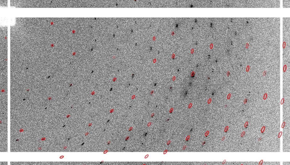 |
| Lattice 02 | 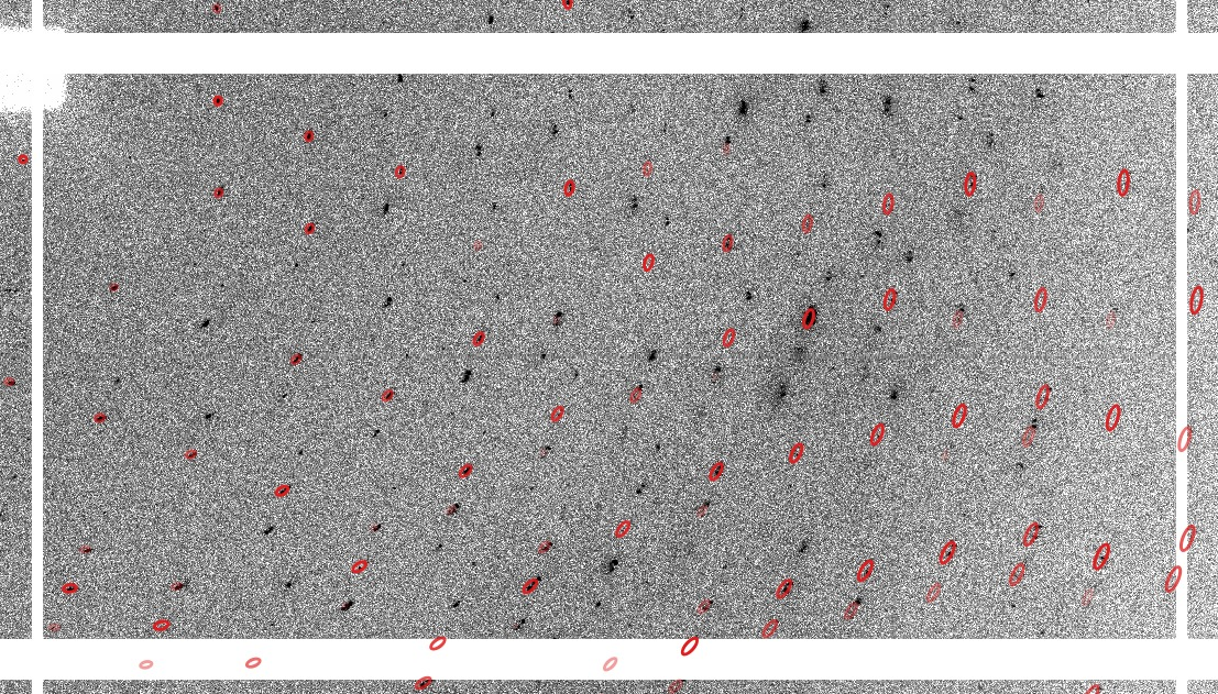 |
| Lattice 03 | 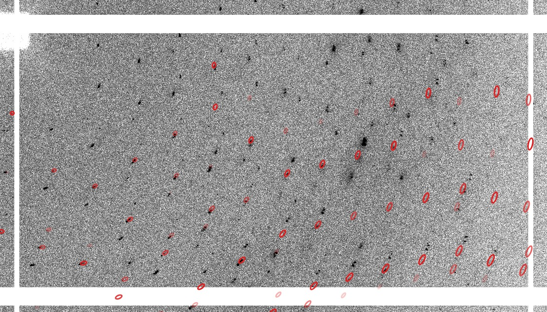 |
| Lattice 04 | 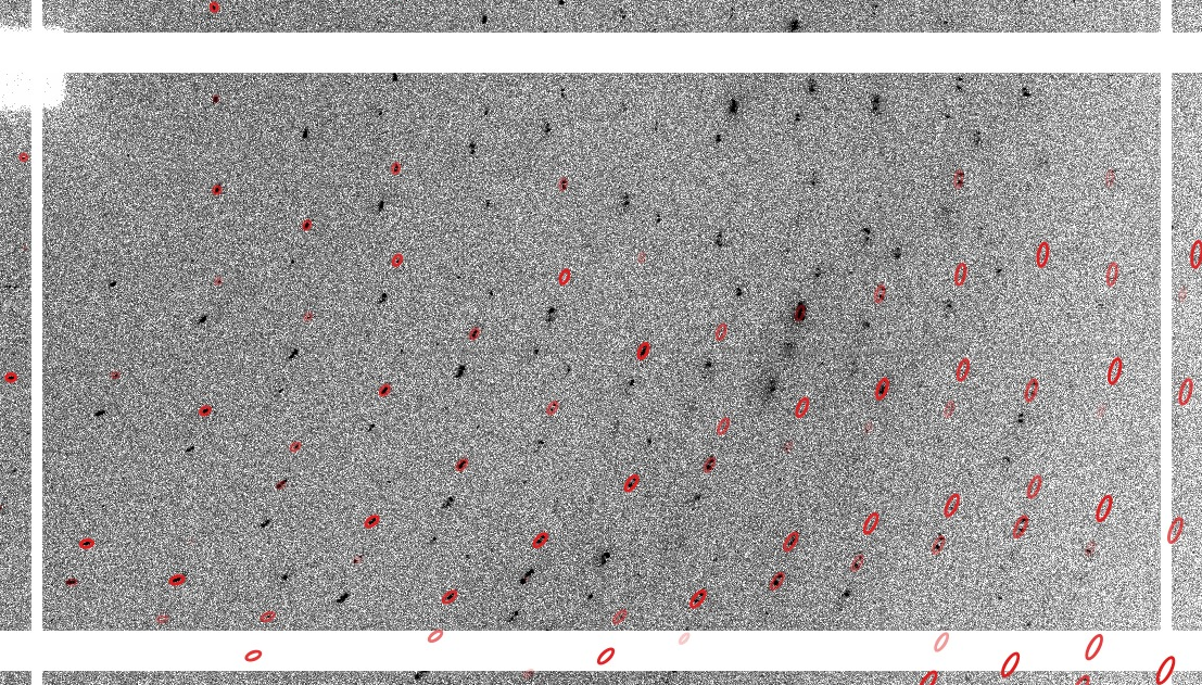 |
which can show you what each indexing solution is predicting.
A more powerful interactive method is to use our own GPX2 visualiser. On standard output you will see various notes
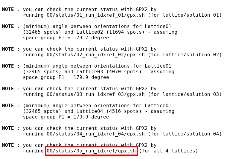 |
Interesting in this case is to follow the last note and run
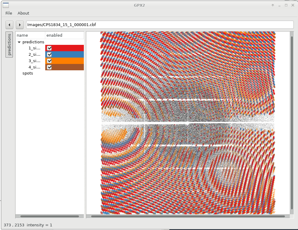
00/status/05_run_idxref/gpx.shwhich will (1) generate predictions for all four indexing solutions (using a default mosaicity value!) and (2) display all orientations simultaneously:
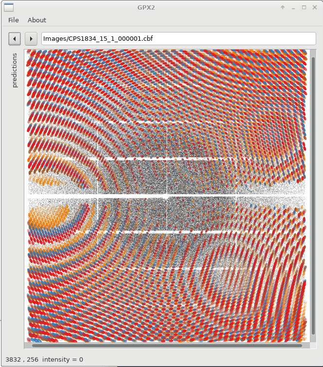 |
We can already see that the different solutions are quite similar (lunes are quite close together), but show some small deviations. We can now switch on/off specific solutions: for that we expand the "predictions" panel (to the left) which then gives us this control. Please note that sometimes you need to double-click on a checkbox to (de)activate a particular prediction.
 |
Zooming in with the scroll-wheel shows us how each indexing solutions picks a different (sub)set of spots, out of the clearly not quite clean, single lattice diffraction observed:
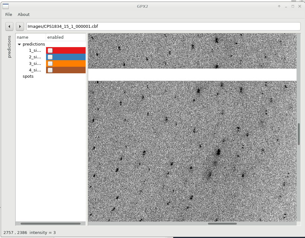 |
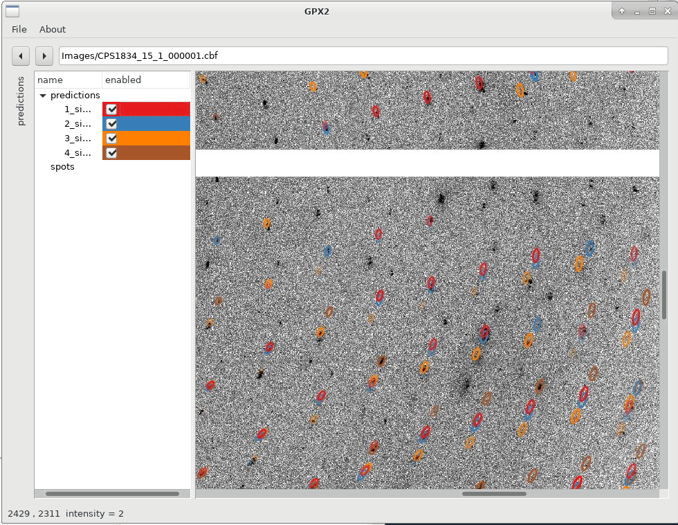 |
The next message deals with (potential) ice-rings:
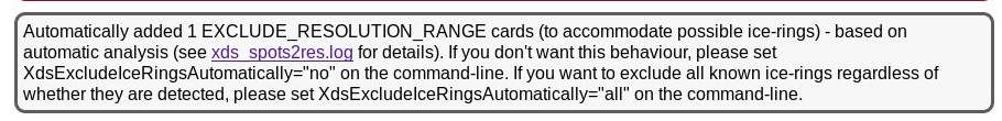 |
So maybe the large number of unindexed spots is due to some ice-rings being present?
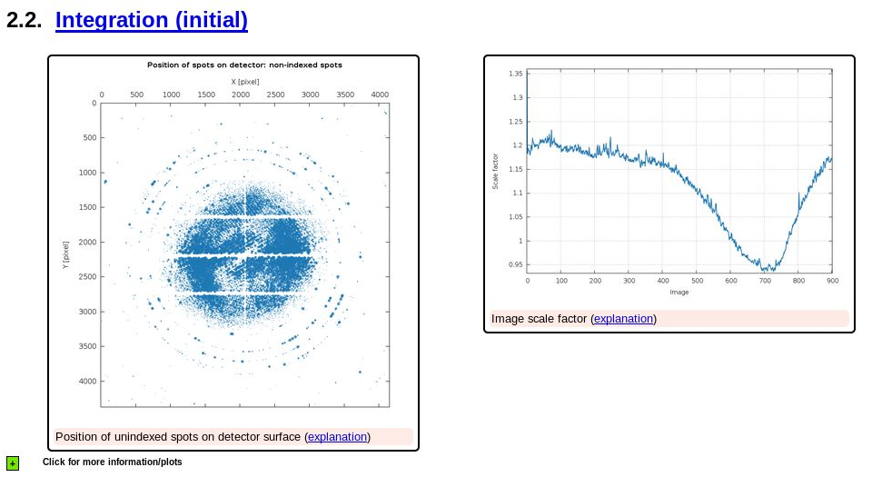 |
shows some (weak) indication of ice-rings, but also still a very large number of spots that are unindexed. There could be all kind of reasons for this, but the most likely is that the poor (in the sense of not being sharp and clean) diffraction leads to poor spot positions - and a lot of spots will just be too far off the predicted reciprocal lattice point to make the cut (into one of the indexing solutions). Still: this is definiteily something to worry about since it shows problems at the spot shape level.
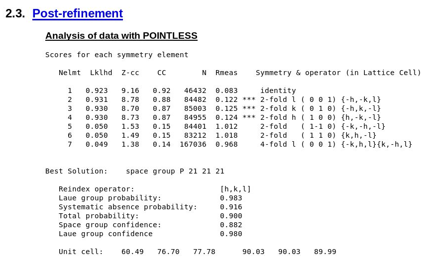
Does this processing job give the same space-group and cell decision as we expect? The deposited structure has cell dimensions
60.370 76.520 77.610 90.00 90.00 90.00 P 21 21 21
and POINTLESS6 gives us indeed
 |
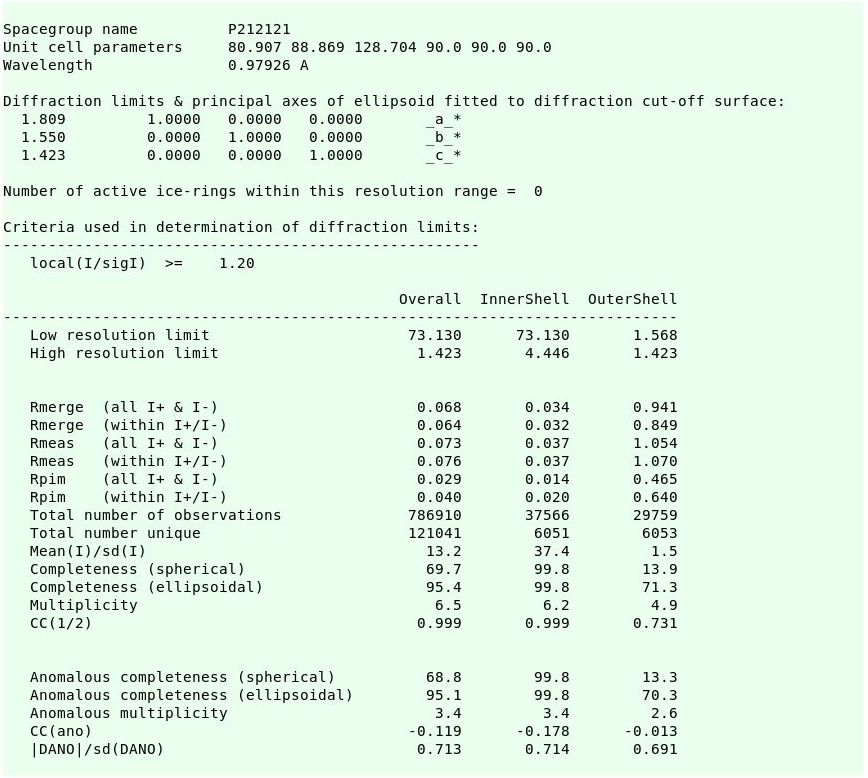
We should now have a closer look at the data quality metrics obtained during scaling and merging of the integrated intensities. First for the data as used in scale determination:
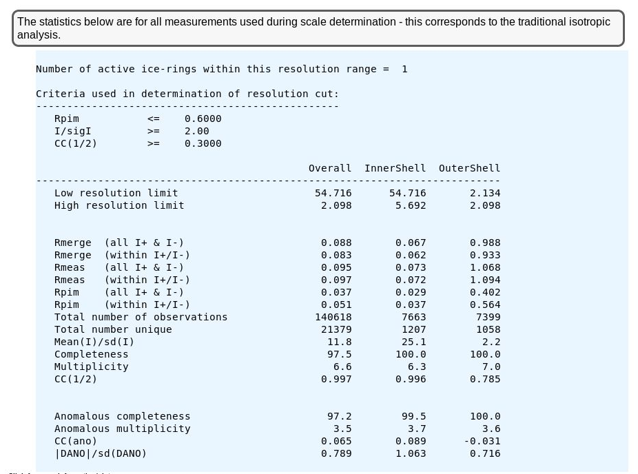 |
This looks ok - similar(ish) to the deposited data as seen in the PDB file
REMARK 200  INTENSITY-INTEGRATION SOFTWARE : XDS
REMARK 200  DATA SCALING SOFTWARE          : AIMLESS
REMARK 200
REMARK 200  NUMBER OF UNIQUE REFLECTIONS   : 16627
REMARK 200  RESOLUTION RANGE HIGH      (A) : 2.300
REMARK 200  RESOLUTION RANGE LOW       (A) : 47.650
REMARK 200  REJECTION CRITERIA  (SIGMA(I)) : NULL
REMARK 200
REMARK 200 OVERALL.
REMARK 200  COMPLETENESS FOR RANGE     (%) : 100.0
REMARK 200  DATA REDUNDANCY                : 7.000
REMARK 200  R MERGE                    (I) : 0.14200
REMARK 200  R SYM                      (I) : NULL
REMARK 200  <I/SIGMA(I)> FOR THE DATA SET  : 10.5000
REMARK 200
REMARK 200 IN THE HIGHEST RESOLUTION SHELL.
REMARK 200  HIGHEST RESOLUTION SHELL, RANGE HIGH (A) : 8.90
REMARK 200  HIGHEST RESOLUTION SHELL, RANGE LOW  (A) : 47.65
REMARK 200  COMPLETENESS FOR SHELL     (%) : NULL
REMARK 200  DATA REDUNDANCY IN SHELL       : 5.80
REMARK 200  R MERGE FOR SHELL          (I) : 0.04800
REMARK 200  R SYM FOR SHELL            (I) : NULL
REMARK 200  <I/SIGMA(I)> FOR SHELL         : NULL
and in the mmCIF file
_reflns.d_resolution_high                2.30
_reflns.d_resolution_low                 47.65
_reflns.number_obs                       16627
_reflns.percent_possible_obs             100.0
_reflns.pdbx_redundancy                  7.0
_reflns.pdbx_Rmerge_I_obs                0.142
_reflns.pdbx_netI_over_sigmaI            10.5
_reflns.pdbx_Rrim_I_all                  0.153
_reflns.pdbx_diffrn_id                   1,2
_reflns.pdbx_ordinal                     1
_reflns.pdbx_CC_half                     0.997
#
loop_
_reflns_shell.d_res_high
_reflns_shell.d_res_low
_reflns_shell.number_unique_obs
_reflns_shell.percent_possible_obs
_reflns_shell.Rmerge_I_obs
_reflns_shell.pdbx_redundancy
_reflns_shell.pdbx_netI_over_sigmaI_obs
_reflns_shell.pdbx_Rrim_I_all
_reflns_shell.pdbx_ordinal
_reflns_shell.pdbx_CC_half
8.90 47.65 341  99.7  0.048 5.8 33.0 0.053 1 0.998
2.30 2.38  1612 100.0 1.216 7.1 1.7  1.312 2 0.664
A bit higher resolution, lower R-merge{footnote:a data quality metric that we should no longer use}, lower Rmeas{footnote same as Rrim} and higher redundancy/multiplicity. Be aware that it is not entirely clear if the deposited data consists of a combination of the inhouse CCD data with this synchrotron PAD data: the _reflns.pdbx_diffrn_id value seems to suggests this, but the lower redundancy somehow contradicts it.
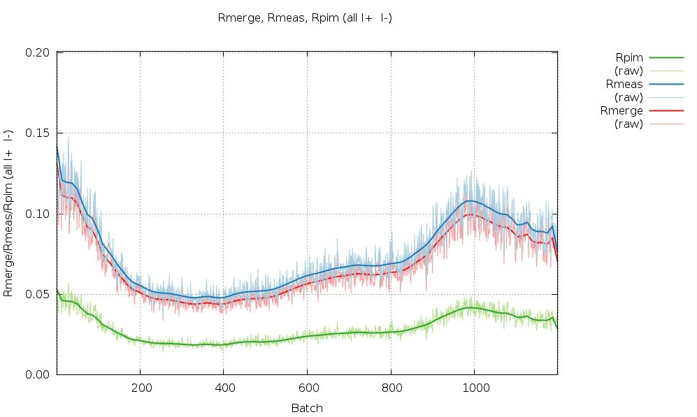
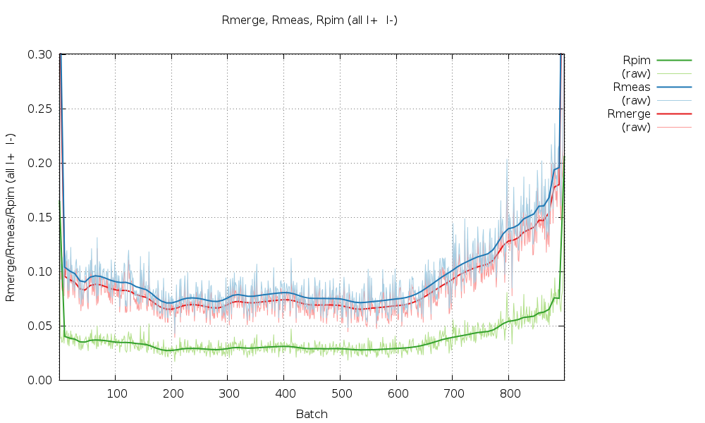
We can look at the statistics graphically by expanding the green "+" symbol. The most interesting ones at the moment are probably those as a function of image number towards the end. The various R-values show some trends as a
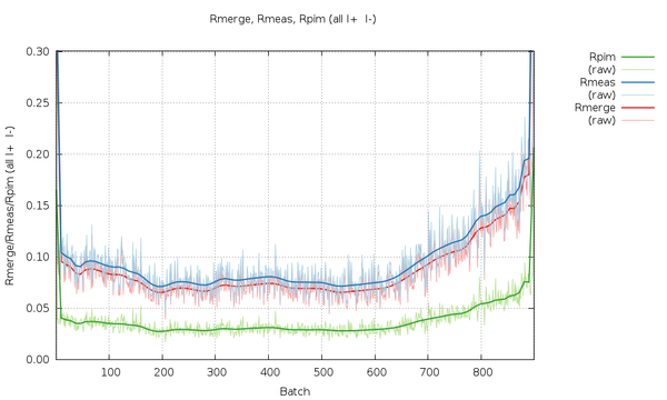 |
All R-values show a so-called "smiley" shape (higher at beginning and end compared to the middle image range. This can often be an indication of radiation damage, i.e. the data collected near the mid-point is most similar to the average (damaged) data - while the early and late data is the most dissimilar. Here the increase at the beginning is not that pronounced, but it definitely rises towards the final third of the dataset.
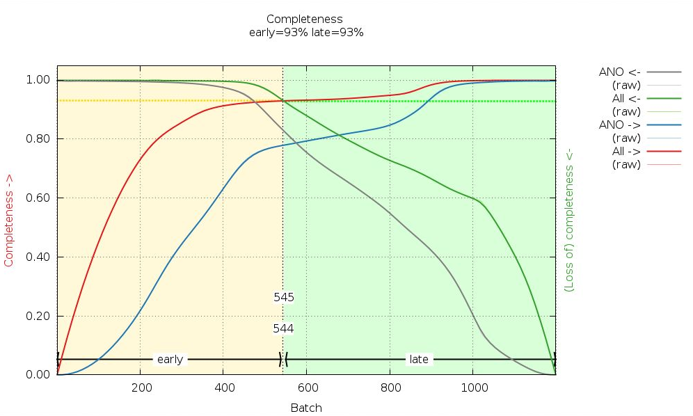
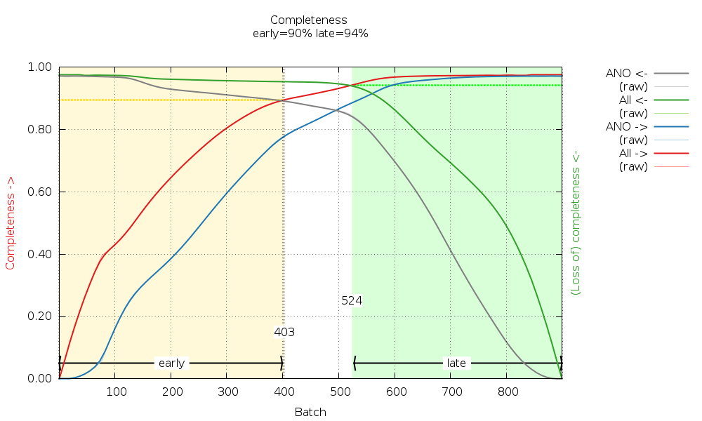
Can we do something about or with this information? Let's look at the cumulative completeness plot:
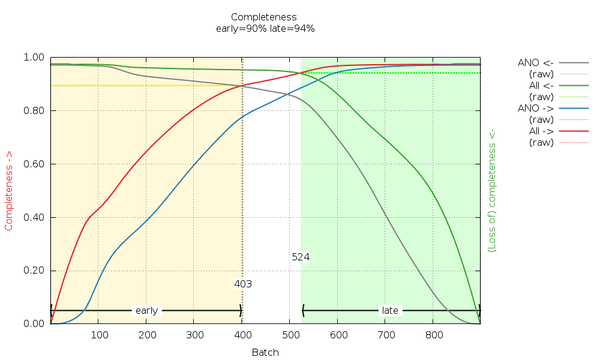 |
We can see that by using images 1-403 and images 524-900 we can generate fairly complete datasets, which we call "early" and "late". These are generated automatically here (by scaling all data together and then merging the early image range and the late image range separately). The reflection data frm the traditional (isotropic) data analysis will contain those F(early) and F(late) amplitudes (truncate-unique.mtz) and can be used in BUSTER for automatic analysis of potential radiation damage effects on the atomic model. We will discuss this in the BUSTER part of this example.
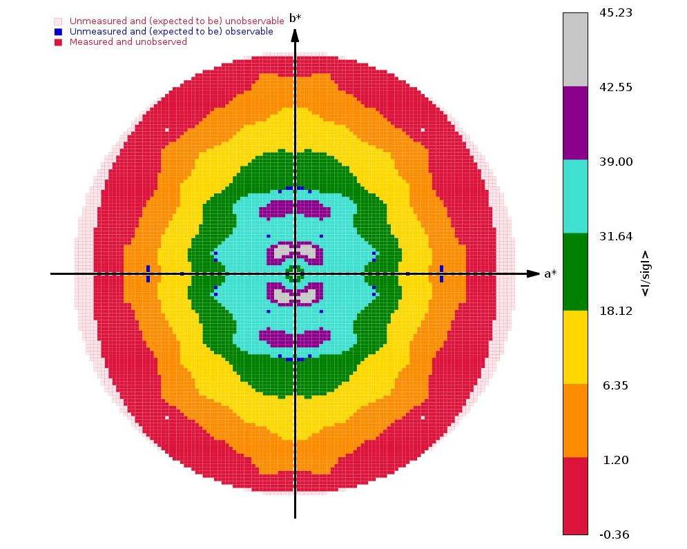
The next interesting analysis has to do with data anisotropy as analysied by STARANISO:
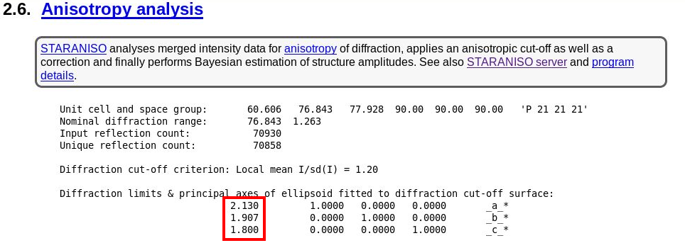 |
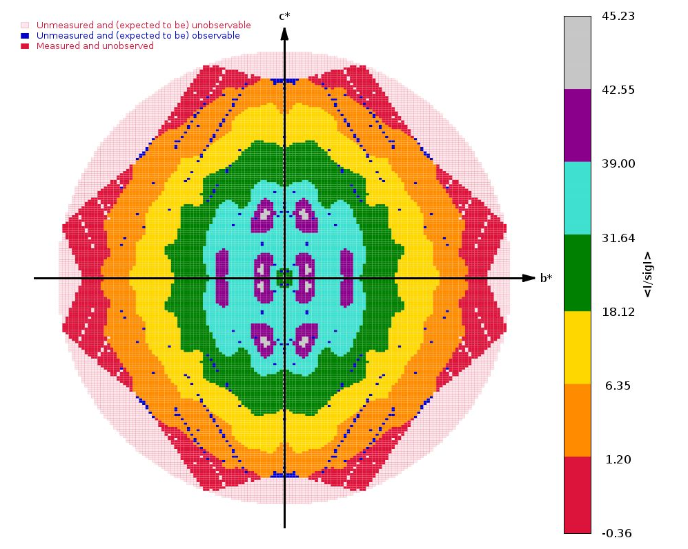
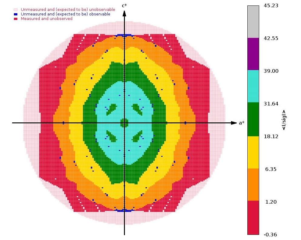
As we can see, there is a slight anisotropy as judged from those principal axes (of the fitted ellipsoid): 1.8A in the best and 2.1A in the worst direction. We can see this effect also in the 2D plane pictures further down:
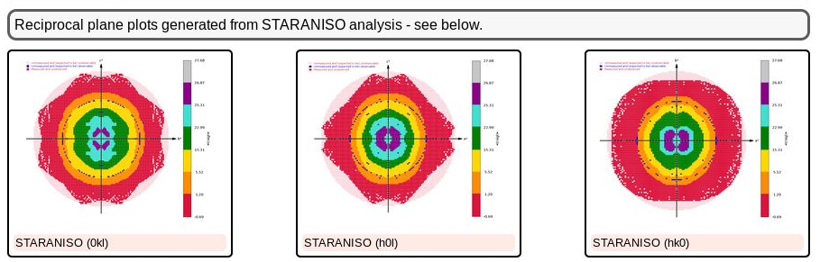 |
What can be seen very nicely here is that the crystal-detector distance was chosen to allow any significant diffraction to be observable: there is a nice red buffer of unobserved (i.e. emasured, but below a significance level) reciprocal lattice points. This means that we won't have lost any significant data due to a too large crystal-detector distance: nice.
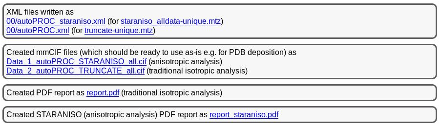
The final results are then again summarised near the bottom:
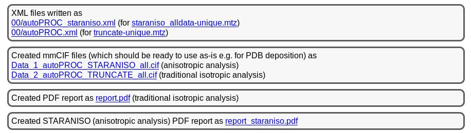 |
You can see that we provide two versions of each type of result (MTZ, mmCIF, XML and PDF), one for the traditional (isotropic) analysis and one for the anisotropic (STARANISO) analysis. Which one to use in subsequent stages might depend on the purpose (experimental phasing, molecular replacement, refinement) or the program used.
This is only 1 of 2 structures related to Covid-19/SARS-CoV2 work for which deposited images are available as of 20200324. So it is a good opportunity to see what can be done with current software and methods on data collected 4 years ago and a model deposited 2.5 years ago). It is great that the authors deposited not only the processed, but also the raw data - thanks a lot!
The raw images are available from SBGrid here7 , e.g. using the command
[ ! -d 5VZR ] && mkdir 5VZR && ( cd 5VZR && rsync -av rsync://data.sbgrid.org/10.15785/SBGRID/496 . ; ln -s 496 Images)
We will leave some of the more detailed explanations and instructions out of this example - they will have been provided in the Example-1 (6VDB) section above.
We know that the data was collected on beamline 19-ID (SBC-CAT) of the APS. Looking at the autoPROC wiki we see that we need to tell autoPROC that the rotation axis is rotating the other direction (relative to the assumed default used in autoPROC) 8 .
We can run autoPROC using
  cd 5VZR
  process ReverseRotationAxis=yes -d 00 | tee 00.lis
and look at both standard output (00.lis) as well as the 00/summary.html file using e.g.
firefox 00/summary.html
There are quite a few warnings about some problematic spots - probably due to some "flickering" pixels:
 |
But this doesn't cause a problem with indexing:
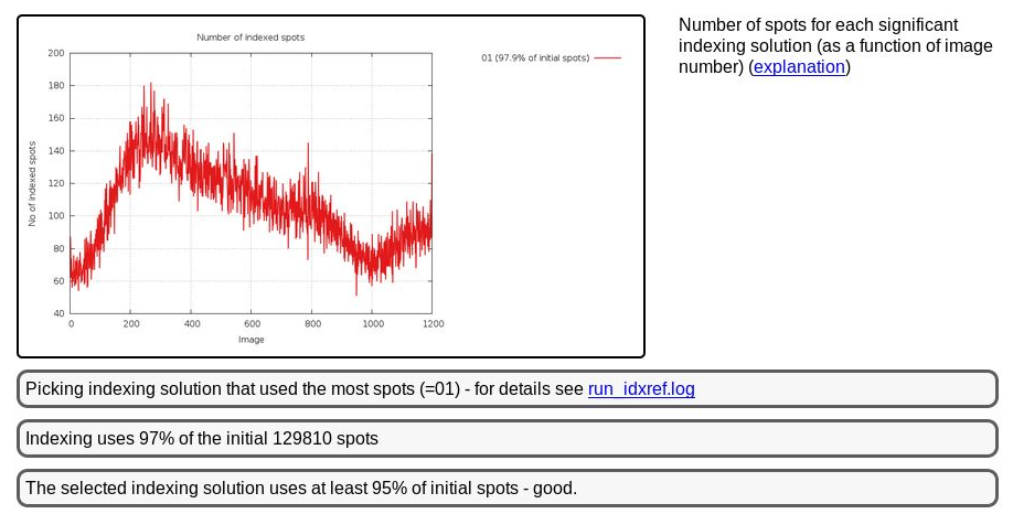 |
There are a few (weak) ice-rings visible - but nothing serious:
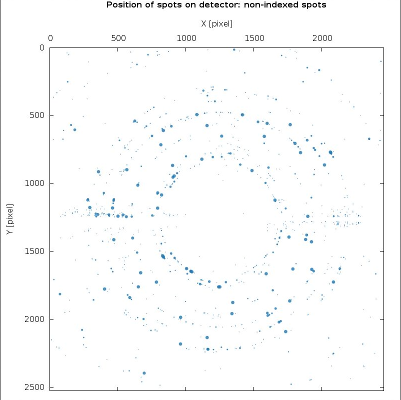 |
We get a warning about unstable distance refinement during the first (in P1) integration run:
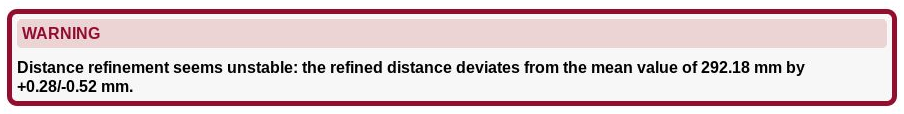 |
If the distance would genuinely move by up to 0.8mm, the crystal would most likely move out of the beam - so this is not what actually happens and the distance refinement is a proxy for something else.
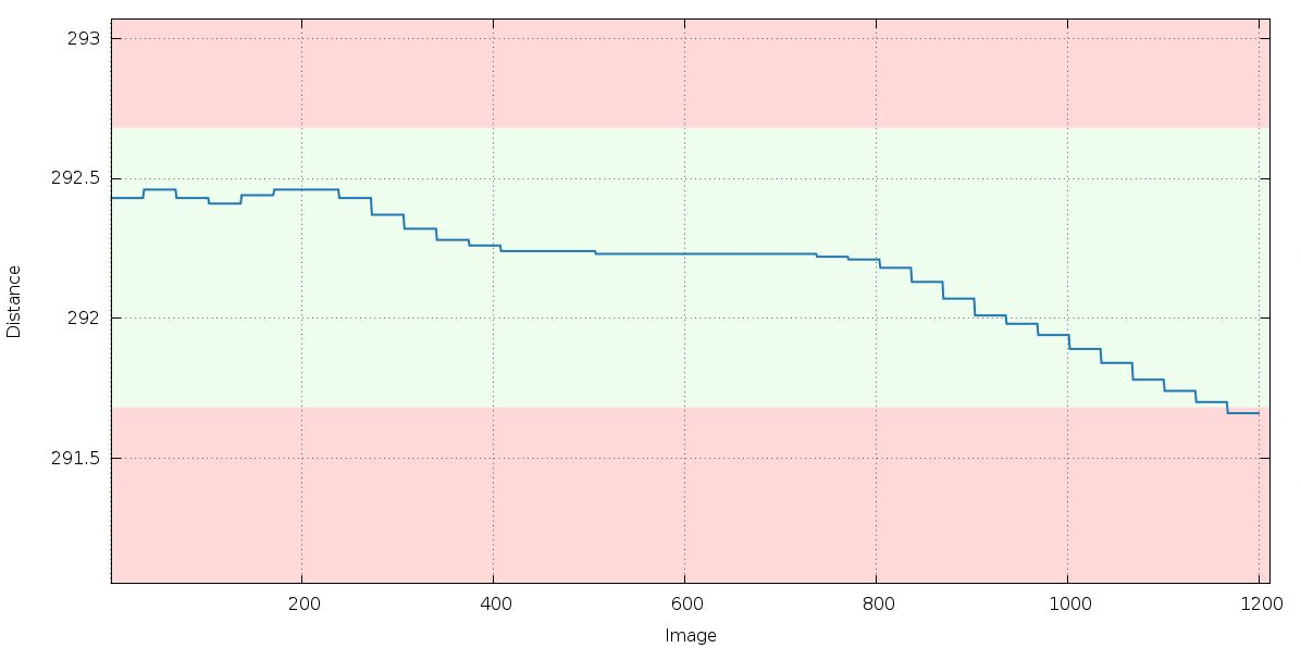 |
Remember that XDS / INTEGRATE will by default keep the cell dimensions fixed and refine the detector position instead. So the above trend could be explained by an increase in cell dimensions (and the distance refinement is trying to accomodate this). This does point to potential radiation damage (which often results in an increase of the unit cell). We'll look at this further down as well.
The symmetry decision in POINTLESS clearly selects the correct SG/cell:
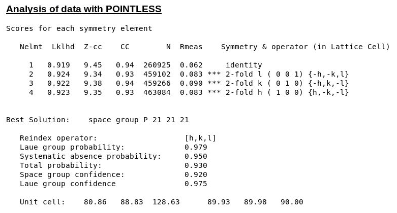 |
The intial step of scale determination (following the traditional isotropic analysis based on - mainly - and average <I/sigma(I)> of 2 in the outer shell) gives
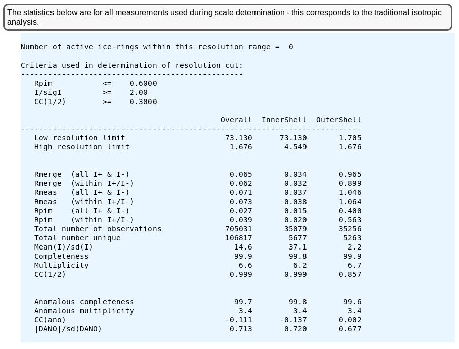 |
which is similar but perhaps consistently better to the original processing statistics:
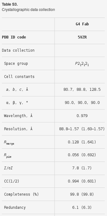 |
We can see that some image ranges are probably better than others - or that there could indeed be radiation damage (remember the distance refinement above?):
 |
 |
We get some clear indications of anisotropy from STARANISO:
 |
 |
 |
resulting in the final scaling and merging statistics:
 |
and files
 |
NOTE: remember that these reflection files contain a (new) random set of test-set flags and for (re-)refinement against the deposited structure the original test-set flags need to be transferred first.
See also BUSTER (re-)refinement follow-up.