Content:
Analysing a dataset/model for radiation damage is important, since we want to know things like (among others):
It is crucial to be aware of the importance of this kind of analysis already at the data collection stage. Low-dose, high-multiplicity (and fine-slicing) strategies on modern beamlines and with modern (PAD) detectors allows for a detailed analysis of radiation-damage metrics (increase in R-values, increase in cell parameters) together with (potentially) restricting the data to a (mostly) undamaged subset of images while still achieving a complete and redundant (i.e. well scaleable) dataset. Furthermore, we can compute F(early)–F(late) maps to visualise the specific radiation damage at the model level (this is done automatically when using autoPROC and BUSTER, but can obviously also be done using other packages/software).
Collecting High-dose, low-multiplicity (mostly a direct effect of using a high dose), wide-sliced data on those new detectors is not a good idea: it damages the samepl/crystal much too fast and uses parameteres that were more adequate for image plate or CCD detectors - and therefore ignore all the benefits of these readout-noise free detectors when run in shutterless mode. We can't see any good reason for not generally following the simple low-dose, high-multiplicity, fine-slicing approach.
F(early)–F(late) maps:
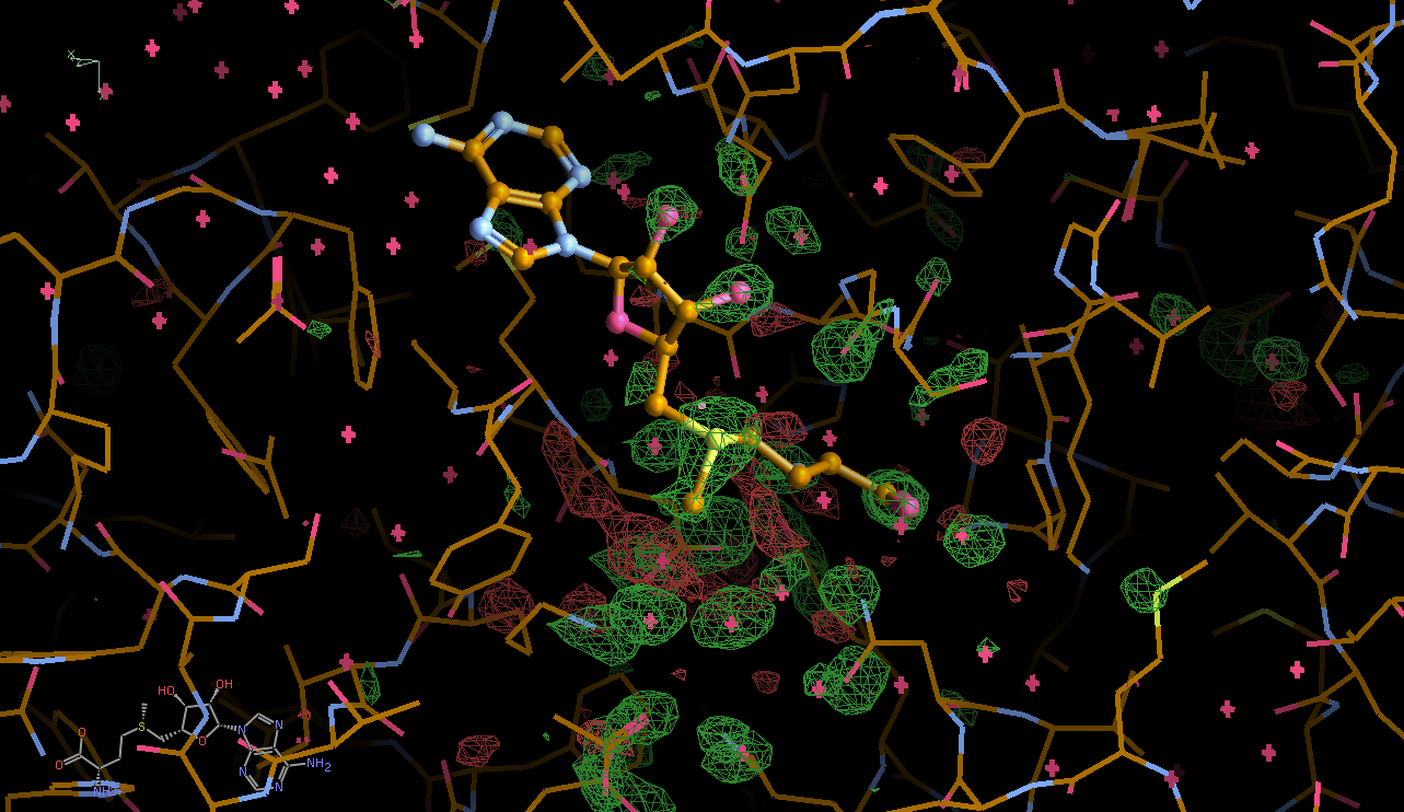
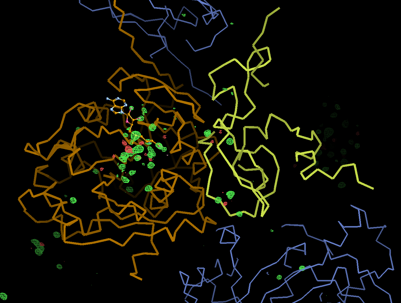
These are normal difference Fourier maps using two sets of amplitudes (from merging an early part of a datasets separately from a late part - as done automatically in autoPROC) and the phases from the current best model refinement. They will show positive density (usually in green if using Coot) where an atom (or atoms) where at the beginning of data collection ("early" amplitudes) and negative density (red) where they might have moved to at the end of data collection ("late"). Of course, atoms/groups are often just disappearing (into the solvent region) without leaving a clear indication of a new and stable location. So it is mostly the positive (green) peaks we are interesting here since these most likely relate to radiation damage (a change relative to the molecule before bombarding it with radiation).
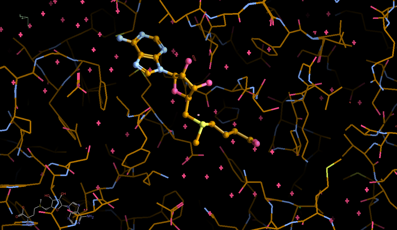
There is a lot going on in the F(early)–F(late) maps - all around the S-Adenosylmethionine residue:

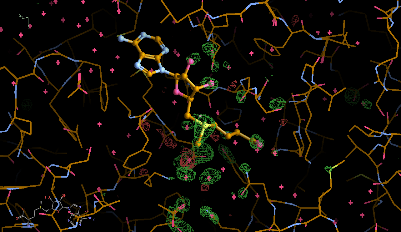
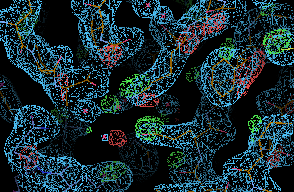
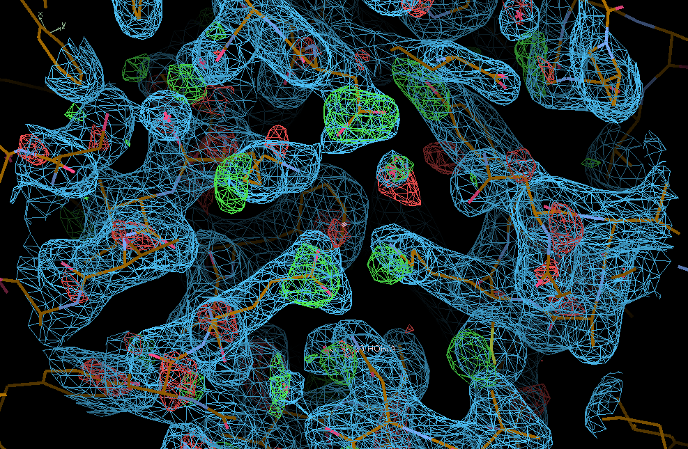
We can break that down a bit in terms of dose - by looking at the gradual changes in four 50-image chunks:
| early/late | 0.50 | 0.75 | 1.00 |
| 0.25 |  |
 |
 |
| 0.50 | 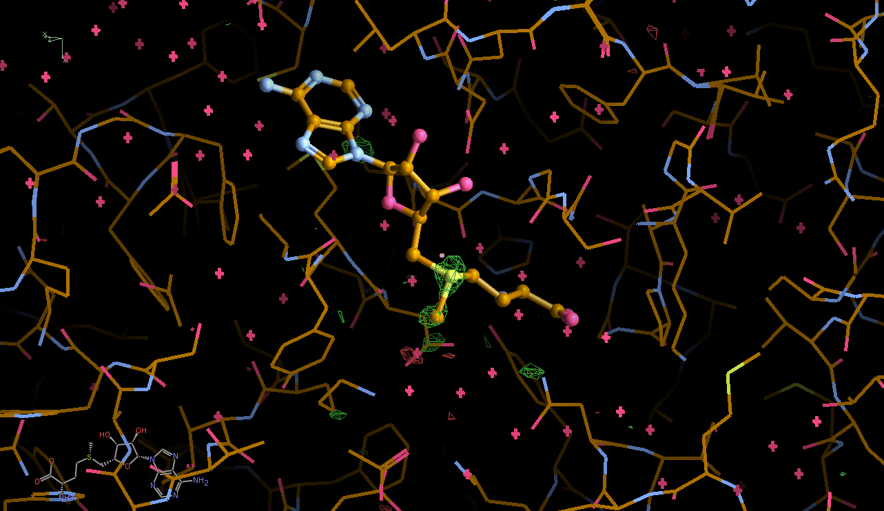 |
 |
|
| 0.75 | 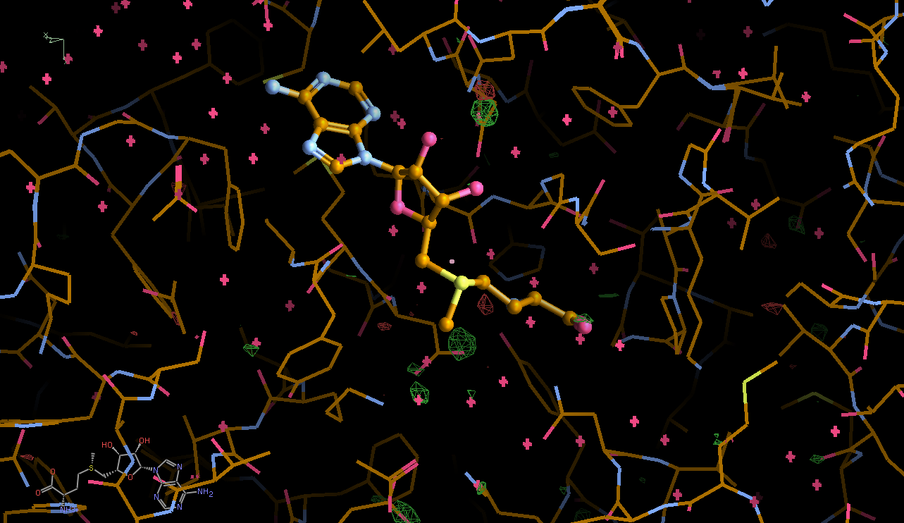 |
This shows that different parts seem to get damaged at different times: decarboxylation, ligand damage, waters moving etc. There is a fair amount of noise in this analysis (should probably done via a sliding window to create a kind of "movie") - mainly because we are not in a position to select complete sections of data with high enough multiplicity (all due to data collection strategy settings).
We can also analyse this different: instead of doing a single refinement (against teh average data) we do individual refinements against each quarter-dataset. But note: these datasets are not the result of processing subset of images independently, but rather of scaling all data together and only splitting it off into separate merged datasets at the final (merging) step. This is an important precedural difference (as done in the aP_scale scaling module of autoPROC), since each individual quarter-dataset would only have a multiplicity of about 1.7-2.1 ... so no real chance of proper scaling and/or outlier rejection. Have we mentioned the benefit of low-dose, high-multiplicity data collection before?
Anyway, the refinements against those quarter datasets produces the following results:
| Dataset | No. of waters | <B> (protein) | <B> SAM |
| 0.25 | 557 | 38.3 | 27.8 |
| 0.50 | 547 | 38.5 | 29.7 |
| 0.75 | 533 | 38.3 | 31.1 |
| 1.00 | 502 | 39.2 | 32.8 |
showing the effect of radiation damage (e.g. decarboxylation) on the water structure we can achieve and the radiation damage on the SAM compound when it comes to atomic B-factors.
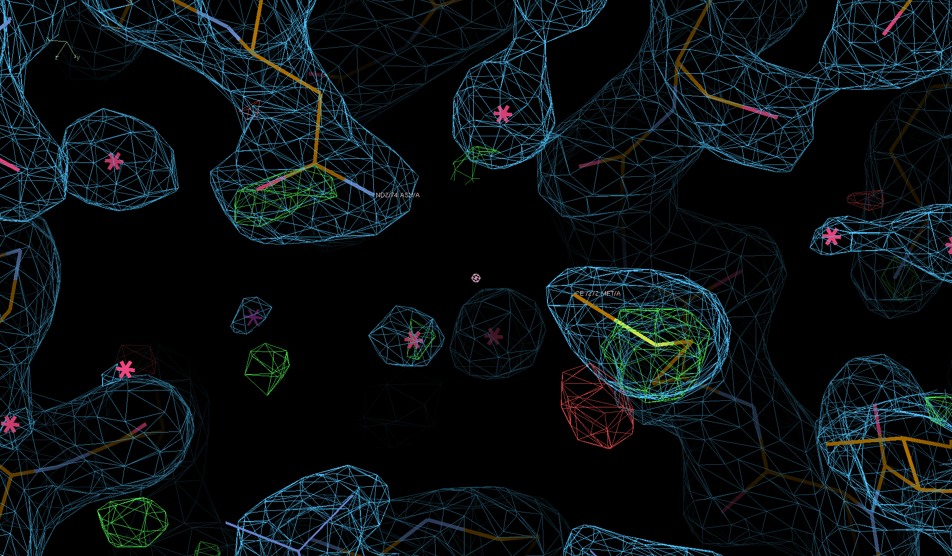
We can see the typical decarboxylation (GLU and ASP residues) as well as damage on Cys/Met sulfurs (also around the Zn site) - with knock-on effects around those residues:
There are some weak indications of radiation damage at
SD  MET A 272
OE1 GLU A  57
OD1 ASP A 268
e.g.: